On the Intuitive Content of Quantum Theoretical Kinematics and Mechanics

Heisenberg, W. Z. Phys. 1927, 43, 172–198. Original German title: “Über den anschaulichen Inhalt der quantentheoretischen Kinematik und Mechanik”

NoteTo the Reader

This is the original 1927 paper in which Werner Heisenberg introduced the uncertainty principle. The 25-year-old physicist showed that certain pairs of physical properties, like position and momentum, cannot both be known precisely at the same time. This limitation is not due to imperfect instruments. It is a fundamental feature of nature at the quantum scale.

For General Chemistry I students, this paper explains why the Bohr model’s precise electron orbits cannot be real. When Heisenberg writes that the “1s orbit of the electron in the hydrogen atom makes no sense,” he is explaining why we must replace orbits with orbitals (probability distributions rather than definite paths). The uncertainty principle, expressed as Δp · Δq ∼ h (equation 1), tells us that the more precisely we know where an electron is, the less precisely we can know its momentum, and vice versa.

The gamma-ray microscope thought experiment in §1 shows why measuring position disturbs momentum. The paper also connects the uncertainty principle to wave-particle duality through de Broglie waves, and concludes that quantum mechanics is inherently statistical. This is not because we lack information, but because nature itself is indeterminate at this scale.

By W. Heisenberg in Copenhagen.

With 2 figures. (Received March 23, 1927.)

Abstract

In the present work, exact definitions of the words position, velocity, energy, etc. (for example, of the electron) are first established that remain valid in quantum mechanics, and it is shown that canonically conjugate quantities can be determined simultaneously only with a characteristic uncertainty (§1).¹ This uncertainty is the actual reason for the occurrence of statistical relationships in quantum mechanics. Its mathematical formulation is achieved through the Dirac-Jordan theory (§2). Proceeding from the principles thus obtained, it is shown how macroscopic processes can be understood from the standpoint of quantum mechanics (§3). To illustrate the theory, several special thought experiments are discussed (§4).

¹ Canonically conjugate quantities are pairs of physical properties whose product has units of action (energy × time). Position and momentum are one such pair; energy and time are another. The uncertainty principle states that these paired quantities cannot both be known precisely at the same time.

Introduction

We believe we understand a physical theory intuitively when we can qualitatively conceive of the experimental consequences of this theory in all simple cases, and when we have simultaneously recognized that the application of the theory never contains internal contradictions.² For example, we believe we understand Einstein’s conception of closed three-dimensional space intuitively because the experimental consequences of this conception are thinkable for us without contradiction. To be sure, these consequences contradict our customary intuitive space-time concepts. But we can convince ourselves that the possibility of applying these customary space-time concepts to very large spaces can be inferred neither from our laws of thought nor from experience.

² “Intuitive” (anschaulich) is the key word in the title. Heisenberg is asking: can we form a mental picture of what quantum mechanics means? Can we visualize it? His answer is yes, but only if we accept that some classical concepts (like “orbit”) must be abandoned or redefined.

The intuitive interpretation of quantum mechanics is still full of internal contradictions, which manifest themselves in the battle of opinions over discontinuum and continuum theory, corpuscles and waves.³ From this alone one might conclude that an interpretation of quantum mechanics with the customary kinematic and mechanical concepts is in any case not possible. Quantum mechanics arose precisely from the attempt to break with those customary kinematic concepts and to put in their place relationships between concrete, experimentally given numbers. Since this appears to have succeeded, the mathematical scheme of quantum mechanics will also need no revision. Equally, a revision of space-time geometry for small spaces and times will not be necessary, since by choosing sufficiently heavy masses we can make the quantum-mechanical laws approximate the classical ones as closely as we like, even when dealing with arbitrarily small spaces and times.

³ This “battle of opinions” refers to the wave-particle duality debate. Is light a wave or a particle? Is an electron a particle or a wave? The answer depends on what experiment you perform. Trying to know both aspects simultaneously runs into fundamental limits.

But that a revision of kinematic and mechanical concepts is necessary seems to follow directly from the fundamental equations of quantum mechanics. When a definite mass m is given, it has a simply understandable meaning in our customary intuition to speak of the position and velocity of the center of mass of this mass m. In quantum mechanics, however, a relation pq − qp = h/2πi between mass, position, and velocity is supposed to hold.⁴ We therefore have good reason to be suspicious of the uncritical application of those words “position” and “velocity.” If one admits that discontinuities are somehow typical of processes in very small spaces and times, then a failure of precisely the concepts “position” and “velocity” is even immediately

⁴ The commutation relation is the mathematical foundation of quantum mechanics. Unlike ordinary algebra where ab = ba, quantum mechanical operators for position (q) and momentum (p) do not commute. Their difference equals h/2πi. This non-commutativity is the mathematical origin of the uncertainty principle.

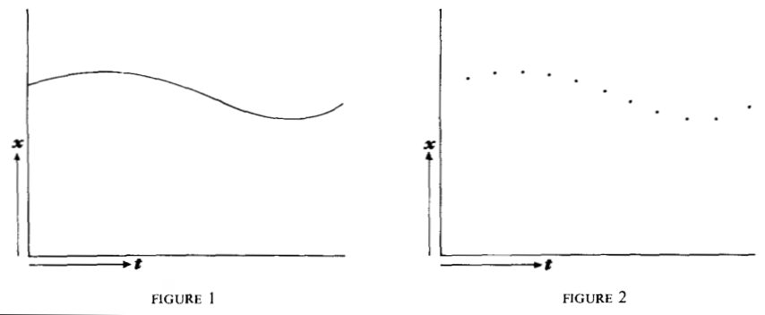
plausible: If one thinks, for example, of the one-dimensional motion of a mass point, then in a continuum theory one will be able to draw a trajectory curve x(t) for the path of the particle (more precisely: its center of mass) (Fig. 1), and the tangent gives the velocity in each case. In a discontinuum theory, however, this curve will perhaps be replaced by a series of points at finite distances (Fig. 2). In this case it is obviously meaningless to speak of the velocity at a particular position, because velocity can only be defined by two positions, and conversely, to each point belong two different velocities.

The question therefore arises whether it might not be possible, through a more precise analysis of those kinematic and mechanical concepts, to clarify the contradictions that have existed until now in the intuitive interpretation of quantum mechanics and to arrive at an intuitive understanding of the quantum-mechanical relations.⁽¹⁾

§1. The Concepts: Position, Path, Velocity, Energy

In order to be able to follow the quantum-mechanical behavior of any object, one must know the mass of this object and the interaction forces with any fields and other objects. Only then can the Hamiltonian function of the quantum-mechanical system be established.⁵ (The following considerations shall generally refer to non-relativistic quantum mechanics, since the laws of quantum-theoretical electrodynamics are still very incompletely known.)⁽²⁾ About the “shape” of the object no further statement is necessary; most appropriately one designates the totality of those interaction forces with the word “shape.”

⁵ The Hamiltonian is a mathematical function that represents the total energy of a system (kinetic + potential). In quantum mechanics, it determines how the system evolves over time. You do not need to understand the mathematics to follow this paper; just know that specifying the Hamiltonian means specifying what forces act on the particle.

If one wants to become clear about what is to be understood by the words “position of the object,” e.g., of the electron (relative to a given reference system), then one must specify definite experiments with whose help one intends to measure the “position of the electron”; otherwise this word has no meaning.⁶ There is no lack of such experiments which in principle allow the “position of the electron” to be determined even to arbitrary precision, e.g.: One illuminates the electron and observes it under a microscope. The highest attainable precision of the position determination is here essentially given by the wavelength of the light used. In principle, however, one could build, say, a γ-ray microscope and carry out the position determination with it as precisely as one wishes.

⁶ Operationalism holds that physical concepts are meaningful only when connected to experimental procedures for measuring them. Heisenberg says: do not ask what position “really is”; ask how you would measure it. This philosophical stance was influential in the development of quantum mechanics.

However, an incidental circumstance is essential in this determination: the Compton effect.⁷ Every observation of the scattered light coming from the electron presupposes a photoelectric effect (in the eye, on the photographic plate, in the photocell), and can therefore also be interpreted as follows: a light quantum⁸ strikes the electron, is reflected or diffracted by it, and then, bent once more by the lenses of the microscope, triggers the photoelectric effect.

⁷ The gamma-ray microscope thought experiment is Heisenberg’s most famous illustration of the uncertainty principle. To see something small, you need short-wavelength light (gamma rays). But shorter wavelength means higher energy photons, and these kick the electron harder when they scatter off it. You can see where the electron was, but you have changed its momentum in the process.

⁸ A light quantum is what we now call a photon. Einstein introduced this term in 1905 to explain the photoelectric effect. It means light comes in discrete packets of energy E = hν, not as a continuous wave. The word “photon” wasn’t coined until 1926.

At the instant of position determination, that is, at the instant when the light quantum is diffracted by the electron, the electron changes its momentum discontinuously.⁹ This change is greater the smaller the wavelength of the light used, i.e., the more precise the position determination is. At the moment when the position of the electron is known, its momentum can therefore only be known up to magnitudes corresponding to that discontinuous change; thus the more precisely the position is determined, the less precisely the momentum is known, and conversely; in this we perceive a direct intuitive illustration of the relation pq − qp = h/2πi.

⁹ Why does momentum change? When a photon bounces off an electron, it transfers some of its momentum (the Compton effect). Higher energy photons (shorter wavelength, better for seeing position) transfer more momentum. The act of observing changes what you’re observing.

Let q₁ be the precision with which the value q is known (q₁ is roughly the mean error of q), thus here the wavelength of the light, and let p₁ be the precision with which the value p can be determined, thus here the discontinuous change of p in the Compton effect; then according to elementary formulas of the Compton effect, p₁ and q₁ stand in the relation

\[p_1 q_1 \sim h \tag{1}\]

That this relation (1) stands in direct mathematical connection with the commutation relation pq − qp = h/2πi will be shown later.¹⁰ Here let it be noted that equation (1) is the precise expression for the facts which one earlier sought to describe by dividing phase space into cells of size h.

¹⁰ Equation (1) is the uncertainty principle in its original form. The product of the uncertainties in position (q₁) and momentum (p₁) is approximately equal to Planck’s constant h. Robertson (1929) later proved the rigorous inequality Δx · Δp ≥ ℏ/2. The essential insight is the same: you cannot make both uncertainties arbitrarily small.

For determining the electron position, one can also perform other experiments, e.g., collision experiments.¹¹ A precise measurement of position requires collisions with very fast particles, since for slow electrons the diffraction phenomena, which according to Einstein are a consequence of de Broglie waves (see, e.g., the Ramsauer effect), prevent a precise determination of position. In a precise position measurement, the momentum of the electron again changes discontinuously, and a simple estimation of the precisions with the formulas for de Broglie waves again gives relation (1).

¹¹ De Broglie waves: In 1924, Louis de Broglie proposed that all matter has wave properties, with wavelength λ = h/p. Slow particles have long wavelengths and diffract around obstacles, making their position fuzzy. Fast particles have short wavelengths and can be localized more precisely.

Through this discussion, the concept “position of the electron” seems clearly enough defined, and only a word need be added about the “size” of the electron. If two very fast particles strike the electron one after the other in a very short time interval Δt, then the positions of the electron defined by the two particles lie very close to each other at a distance Δl. From the laws observed for α-rays, we conclude that Δl can be reduced to magnitudes of the order of 10⁻¹² cm, if only Δt is chosen sufficiently small and the particles sufficiently fast. This is the meaning when we say that the electron is a corpuscle whose radius is not larger than 10⁻¹² cm.

Let us now turn to the concept “path of the electron.” By path we understand a series of spatial points (in a given reference system) which the electron assumes as “positions” one after another. Since we already know what is to be understood by “position at a definite time,” no new difficulties arise here. Nevertheless, it is easy to see that, for example, the often-used expression, the “1s orbit of the electron in the hydrogen atom,” has no meaning from our point of view.¹² For to measure this 1s “orbit,” the atom would have to be illuminated with light whose wavelength is in any case considerably shorter than 10⁻⁸ cm. But from such light, a single light quantum is sufficient to throw the electron completely out of its “orbit” (which is why only a single spatial point of such an orbit can ever be defined); the word “orbit” therefore has no reasonable meaning here. This can be inferred simply from the experimental possibilities, without knowledge of the newer theories.

¹² This is why chemistry uses orbitals, not orbits. The Bohr model’s circular paths cannot be observed because any attempt to observe them would destroy the atom. The electron does not have a definite trajectory. Quantum mechanics gives us probability distributions describing where the electron is likely to be found.

On the other hand, the contemplated position measurement can be carried out on many atoms in the 1S state. (Atoms in a given “stationary” state can in principle be isolated, e.g., by the Stern-Gerlach experiment.)¹³¹⁴ Thus for a definite state, e.g., 1S, of the atom, there must be a probability function for the positions of the electron, which corresponds to the mean value of the classical orbit over all phases and which can be established by measurements with arbitrary precision. According to Born,⁽³⁾ this function is given by ψ₁ₛ(q)ψ₁ₛ(q), where ψ₁ₛ(q) denotes the Schrödinger wave function belonging to state 1S.¹⁵ With Dirac and Jordan, I would like to say with a view to later generalizations: The probability is given by S(1S, q)S(1S, q), where S(1S, q) denotes that column of the transformation matrix S(E, q) from E to q which belongs to E = E₁ₛ.

¹³ The Stern-Gerlach experiment (1922) passed a beam of silver atoms through an inhomogeneous magnetic field. The beam split into two, demonstrating that atomic angular momentum (and later, electron spin) is quantized. This experiment allows atoms in specific quantum states to be separated and studied.

¹⁴ A stationary state is what Gen Chem calls an “energy level.” The electron in hydrogen’s 1S state has n = 1. Heisenberg uses “stationary” because the energy does not change over time (unless the atom absorbs or emits light). The term comes from the Bohr model, where electrons in allowed orbits do not radiate.

¹⁵ The Born interpretation of the wave function. The wave function ψ does not directly tell us where the electron is. Instead, |ψ|² (the wave function multiplied by its complex conjugate) gives the probability density for finding the electron at each location. This is the ψ² you see in orbital diagrams.

In the fact that in quantum theory only the probability function of the electron position can be given for a definite state, e.g., 1S, one may perceive with Born and Jordan a characteristically statistical feature of quantum theory in contrast to classical theory. But one can also say with Dirac, if one wishes, that the statistics are brought in by our experiments.¹⁶ For obviously even in classical theory only the probability of a definite electron position would be specifiable as long as we do not know the phases of the atom. The difference between classical and quantum mechanics consists rather in this: Classically we can always imagine the phase to be determined by preceding experiments. In reality, however, this is impossible because every experiment for determining the phase destroys or changes the atom. In a definite stationary “state” of the atom, the phases are undetermined in principle, which one can regard as a direct illustration of the familiar equations

¹⁶ Quantum probability is not classical probability. The statistical nature of quantum mechanics is not due to ignorance of hidden information (as in classical statistical mechanics). The information simply does not exist. The phases (where the electron is in its orbit) are not unknown; they are indeterminate.

\[\mathbf{E}t - t\mathbf{E} = \frac{h}{2\pi i} \quad \text{or} \quad \mathbf{J}w - w\mathbf{J} = \frac{h}{2\pi i}\]

(J = action variable, w = angle variable.)¹⁷

¹⁷ Action variables (J) and angle variables (w) come from classical mechanics. For Gen Chem purposes: J encodes “which energy level” (related to quantum number n), and w encodes “where the electron is in its orbit” (the phase). The uncertainty relation Jw ~ h says: if you know the energy precisely, you cannot know where in the orbit the electron is. This is why stationary states have definite energy but no definite electron position.

The word “velocity” of an object can easily be defined through measurements when dealing with force-free motion.¹⁸ One can, for example, illuminate the object with red light and determine the velocity of the particle from the Doppler effect of the scattered light. The determination of velocity becomes more precise the longer the wavelength of the light used, since then the velocity change of the particle per light quantum through the Compton effect becomes smaller. The position determination becomes correspondingly imprecise, in accordance with equation (1).

¹⁸ Doppler effect measurements use longer wavelength light (like red light) to measure velocity more precisely. The tradeoff is exactly opposite to position measurement: longer wavelengths disturb momentum less but give worse position information. This is the uncertainty principle in action.

If the velocity of the electron in the atom is to be measured at a definite instant, one will, say, at this instant let the nuclear charge and the forces from the other electrons suddenly disappear, so that the motion from then on is force-free, and will then carry out the determination described above. Again one can easily convince oneself, as above, that a function p(t) cannot be defined for a given state of an atom, e.g., 1S. However, there is again a probability function for p in this state, which according to Dirac and Jordan has the value S(1S, p)S(1S, p). S(1S, p) again denotes that column of the transformation matrix S(E, p) from E to p which belongs to E = E₁ₛ.

Finally, let us point to experiments which allow the measurement of the energy or the values of the action variables J; such experiments are especially important because only with their help can we define what we mean when we speak of the discontinuous change of energy and of J.¹⁹ The Franck-Hertz collision experiments allow the energy measurement of atoms, because of the validity of the conservation of energy in quantum theory, to be reduced to the energy measurement of electrons moving in a straight line. This measurement can in principle be carried out with arbitrary precision, if only one foregoes the simultaneous determination of the electron position, i.e., the phase, in accordance with the relation Et − tE = h/2πi.

¹⁹ The Franck-Hertz experiment (1914) showed that atoms can only absorb energy in discrete amounts. Electrons passing through mercury vapor lost energy in fixed increments of 4.9 eV, corresponding to the energy needed to excite mercury atoms. This was direct experimental proof of quantized energy levels.

The Stern-Gerlach experiment allows the determination of the magnetic or an average electric moment of the atom, thus the measurement of quantities that depend only on the action variables J. The phases remain undetermined in principle. Just as it makes no sense to speak of the frequency of a light wave at a definite instant, one cannot speak of the energy of an atom at a definite moment.²⁰

²⁰ Why can’t we speak of energy at a definite instant? Just as a musical note requires time to establish its frequency (a brief click has no definite pitch), an atom requires time to establish its energy. This is the energy-time uncertainty relation.

Correspondingly, in the Stern-Gerlach experiment the precision of energy measurement decreases the shorter the time span during which the atoms are under the influence of the deflecting force.⁽⁴⁾ An upper limit for the deflecting force is given by the fact that the potential energy of that deflecting force within the beam can only vary by amounts that are considerably smaller than the energy differences of the stationary states, if a determination of the energy of the stationary states is to be possible. Let E₁ be an energy amount that satisfies this condition (E₁ simultaneously gives the precision of that energy measurement); then E₁/d is the maximum value of the deflecting force, where d denotes the width of the beam (measurable through the aperture of the slit used). The angular deflection of the atomic beam is then E₁t₁/dp, where t₁ denotes the time span during which the atoms are under the influence of the deflecting force, and p the momentum of the atoms in the beam direction.

This deflection must be at least of the same order of magnitude as the natural broadening of the beam caused by diffraction at the aperture, for a measurement to be possible. The angular deflection through diffraction is approximately λ/d, where λ denotes the de Broglie wavelength, thus

\[\frac{\lambda}{d} \sim \frac{E_1 t_1}{dp} \quad \text{or, since} \quad \lambda = \frac{h}{p}\]

\[E_1 t_1 \sim h \tag{2}\]

This equation corresponds to equation (1) and shows how a precise energy determination can only be achieved through a corresponding imprecision in time.²¹

²¹ Equation (2) is the energy-time uncertainty relation. To measure an energy precisely, you need to observe the system for a long time. A short observation gives only a rough energy measurement. This explains why spectral lines from short-lived excited states are broadened.

§2. The Dirac-Jordan Theory

One would like to summarize and generalize the results of the preceding section in this assertion: All concepts that are used in classical theory for the description of a mechanical system can also be defined exactly for atomic processes analogously to the classical concepts.²² However, the experiments that serve such a definition carry, purely empirically, an uncertainty within themselves when we demand from them the simultaneous determination of two canonically conjugate quantities. The degree of this uncertainty is given by relation (1) (extended to any canonically conjugate quantities).

²² Section preview. What follows is a mathematical demonstration that the uncertainty principle emerges naturally from the mathematics of quantum mechanics. For Gen Chem students, the key point is that this is not just a practical limitation on our instruments. The uncertainty is built into the mathematical structure of the theory itself.

It is natural here to compare quantum theory with special relativity. According to relativity theory, the word “simultaneous” cannot be defined other than through experiments in which the propagation velocity of light enters essentially. If there existed a “sharper” definition of simultaneity, e.g., signals that propagate infinitely fast, then relativity theory would be impossible. But because there are no such signals, because rather the speed of light already appears in the definition of simultaneity, room is created for the postulate of the constant speed of light; therefore this postulate does not contradict the meaningful use of the words “position, velocity, time.”

The situation is similar with the definition of the concepts “position of an electron” and “velocity” in quantum theory. All experiments that we can use for the definition of these words necessarily contain the uncertainty specified by equation (1), even though they allow the individual concept p, q to be defined exactly. If there existed experiments that simultaneously allowed a “sharper” determination of p and q than corresponds to equation (1), then quantum mechanics would be impossible. This uncertainty, which is fixed by equation (1), thus first creates room for the validity of the relations that find their most concise expression in the quantum-mechanical commutation relations

\[\mathbf{p}\mathbf{q} - \mathbf{q}\mathbf{p} = \frac{h}{2\pi i}\]

it makes this equation possible without requiring that the physical meaning of the quantities p and q be changed.

For those physical phenomena whose quantum-theoretical formulation is still unknown (e.g., electrodynamics), equation (1) represents a demand that may be useful for finding the new laws. For quantum mechanics, equation (1) can be derived from the Dirac-Jordan formulation through a minor generalization.

If for a definite value η of some parameter we determine the position q of the electron to be q′ with a precision q₁, we can express this fact through a probability amplitude S(η, q) that is appreciably different from zero only in a region of approximate size q₁ around q′. In particular, one can, for example, set²³

²³ What equations (3) through (6) show: Heisenberg proves mathematically that if you know position precisely (small q₁), the momentum must be spread out (large p₁), and vice versa. The product p₁q₁ always equals h/2π. This is not a limitation of our instruments. It emerges unavoidably from the mathematical structure of quantum mechanics.

\[S(\eta, q) \propto e^{-\frac{(q-q')^2}{2q_1^2} - \frac{2\pi i}{h}p'(q-q')}, \quad \text{thus} \quad S\bar{S} \propto e^{-\frac{(q-q')^2}{q_1^2}} \tag{3}\]

Then for the probability amplitude belonging to p:

\[S(\eta, p) = \int S(\eta, q) \, S(q, p) \, dq \tag{4}\]

For S(q, p) one can set, according to Jordan:

\[S(q, p) = e^{\frac{2\pi i p q}{h}} \tag{5}\]

Then according to (4), S(η, p) will be appreciably different from zero only for values of p for which 2π(p − p′)q₁/h is not substantially greater than 1. In particular, in case (3):

\[S(\eta, p) \propto \int e^{\frac{2\pi i(p-p')q}{h} - \frac{(q'-q)^2}{2q_1^2}} \, dq\]

i.e.,

\[S(\eta, p) \propto e^{-\frac{(p-p')^2}{2p_1^2} + \frac{2\pi i}{h}q'(p-p')}, \quad \text{thus} \quad S\bar{S} \propto e^{-\frac{(p-p')^2}{p_1^2}}\]

where

\[p_1 q_1 = \frac{h}{2\pi} \tag{6}\]

The assumption (3) for S(η, q) thus corresponds to the experimental fact that the value p′ for p and the value q′ for q were measured [with the precision limitation (6)].²⁴

²⁴ The math forces the tradeoff. If you start with a wave function narrowly peaked at position q′, then when you transform to momentum space, the resulting function is necessarily spread out. The narrower the position peak, the wider the momentum spread. Their product equals h/2π. This is not a choice; it is a mathematical consequence of how position and momentum representations are related.

From a purely mathematical standpoint, what is characteristic of the Dirac-Jordan formulation of quantum mechanics is that the relations between p, q, E, etc. can be written as equations between very general matrices, such that any given quantum-theoretical quantity appears as a diagonal matrix. The possibility of such a notation is evident when one pictures the matrices intuitively as tensors (e.g., moments of inertia) in multidimensional spaces, between which mathematical relationships exist. One can always orient the axes of the coordinate system in which one expresses these mathematical relationships along the principal axes of one of these tensors.

Finally, one can also always characterize the mathematical relationship between two tensors A and B through the transformation formulas that convert a coordinate system oriented along the principal axes of A into another oriented along the principal axes of B. The latter formulation corresponds to Schrödinger’s theory. As the actual “invariant” formulation of quantum mechanics, independent of all coordinate systems, one will instead regard Dirac’s notation of q-numbers.

If we want to derive physical results from that mathematical scheme, we must assign numbers to the quantum-theoretical quantities, i.e., to the matrices (or “tensors” in multidimensional space). This is to be understood as follows: in that multidimensional space a definite direction is arbitrarily prescribed (namely, determined by the type of experiment performed), and one asks what the “value” of the matrix (e.g., in that picture, the value of the moment of inertia) is in this prescribed direction. This question has a unique meaning only when the prescribed direction coincides with the direction of one of the principal axes of that matrix; in this case there is an exact answer to the question posed.

But even when the prescribed direction deviates only slightly from one of the principal axes of the matrix, one can still speak of the “value” of the matrix in the prescribed direction with a certain imprecision given by the relative inclination, with a certain probable error.²⁵ One can therefore say: Every quantum-theoretical quantity or matrix can be assigned a number indicating its “value” with a definite probable error; the probable error depends on the coordinate system; for every quantum-theoretical quantity there exists a coordinate system in which the probable error for this quantity vanishes.

²⁵ Measurement creates knowledge at the cost of other knowledge. Choosing to measure position precisely means accepting uncertainty about momentum. This is not a flaw in our technique. It is how nature works at the quantum scale.

A definite experiment can thus never give exact information about all quantum-theoretical quantities; rather, it divides the physical quantities into “known” and “unknown” (or: more and less precisely known quantities) in a manner characteristic of the experiment. The results of two experiments can only be derived exactly from each other if the two experiments divide the physical quantities in the same way into “known” and “unknown.” If two experiments bring about different divisions into “known” and “unknown,” then the connection between the results of those experiments can only be stated statistically.

For a more precise discussion of this statistical connection, let us perform a thought experiment.²⁶ Let a Stern-Gerlach atomic beam first be sent through a field F₁ that is so strongly inhomogeneous in the beam direction that it causes appreciably many transitions through “shaking action.” Then let the atomic beam run freely for a while; at a definite distance from F₁, however, let a second field F₂ begin, similarly inhomogeneous to F₁. Between F₁ and F₂ and behind F₂, let it be possible to measure the number of atoms in the various stationary states through a possibly applied magnetic field. Let the radiation forces of the atoms be set to zero.

²⁶ What equations (7) and (8) demonstrate: Heisenberg imagines sending atoms through two regions (F₁ and F₂) that can change their quantum states. The key result: if you measure the atom’s state between the two regions, you get different final probabilities than if you don’t measure. The act of measurement changes the outcome. This is not because measurement is clumsy. Measurement fundamentally alters the quantum state.

If we know that an atom was in the state of energy Eₙ before it passed F₁, we can express this experimental fact by assigning to the atom a wave function—e.g., in p-space—with the definite energy Eₙ and indefinite phase βₙ

\[S(E_n, p) = \psi(E_n, p) \, e^{\frac{2\pi i E_n(t + \beta_n)}{h}}\]

After passing through field F₁, this function will have transformed into⁽⁵⁾

\[S(E_n, p) \to \sum_m c_{nm} \psi(E_m, p) \, e^{\frac{2\pi i E_m(t + \beta_m)}{h}} \tag{7}\]

Here let the βₘ be arbitrarily fixed, so that the cₙₘ are uniquely determined by F₁. The matrix cₙₘ transforms the energy values before passage through F₁ to those after passage through F₁. If we perform a determination of stationary states behind F₁, e.g., through an inhomogeneous magnetic field, we will find with probability cₙₘcₙₘ that the atom has transitioned from state n to state m.

If we experimentally determine that the atom has actually transitioned to state m, then for calculating everything that follows we must assign to it not the function ΣₘcₙₘSₘ but rather the function Sₘ with indefinite phase; through the experimental determination “state m” we select from the multitude of different possibilities (cₙₘ) a definite one: m, but simultaneously destroy, as will be explained later, everything that was still contained in the quantities cₙₘ in terms of phase relationships.

When the atomic beam passes through F₂, the same thing repeats as at F₁. Let dₘₗ be the coefficients of the transformation matrix that transforms the energies before F₂ to those after F₂. If no determination of state is made between F₁ and F₂, then the eigenfunction transforms according to the following scheme:²⁷

²⁷ An eigenfunction (or wave function) is a mathematical function that describes a quantum state. For an electron in an atom, each energy level has its own eigenfunction. The 1s, 2s, 2p orbitals you see in Gen Chem are visualizations of these eigenfunctions. The word comes from German eigen meaning “own” or “characteristic.”

\[S(E_n, p) \xrightarrow{F_1} \sum_m c_{nm} S(E_m, p) \xrightarrow{F_2} \sum_m \sum_l c_{nm} d_{ml} S(E_l, p) \tag{8}\]

Let Σₘcₙₘdₘₗ = eₙₗ. If the stationary state of the atom is determined behind F₂, one will find state l with probability eₙₗeₙₗ. If, on the other hand, the determination “state m” was made between F₁ and F₂, then the probability for “l” behind F₂ will be given by dₘₗdₘₗ. With multiple repetition of the whole experiment (with the state being determined between F₁ and F₂ each time), one will thus observe state l behind F₂ with relative frequency

\[Z_{nl} = \sum_m c_{nm}\bar{c}_{nm} d_{ml}\bar{d}_{ml}\]

This expression does not agree with eₙₗeₙₗ. Jordan (l.c.) has therefore spoken of an “interference of probabilities.” But I would not like to agree with this. For the two experiments that lead to eₙₗeₙₗ or Zₙₗ are indeed physically really different. In one case the atom experiences no disturbance between F₁ and F₂; in the other it is disturbed by the apparatus that enables a determination of the stationary state. This apparatus has the consequence that the “phase” of the atom changes by amounts that are in principle uncontrollable, just as the momentum changes in a determination of electron position (cf. §1).²⁸

²⁸ Phase here does not mean solid/liquid/gas. In physics, phase describes where a wave is in its cycle (like the hands of a clock). Two waves are “in phase” if their peaks align. Quantum mechanically, the phase of a wave function affects how it interferes with other wave functions. Measuring the atom’s energy destroys information about its phase, and vice versa.

The magnetic field for determining the state between F₁ and F₂ will detune the eigenvalues E; in observing the path of the atomic beam (I am thinking, say, of Wilson chamber photographs)²⁹ the atoms are braked statistically differently and uncontrollably, etc.

²⁹ A Wilson cloud chamber (invented 1911) makes particle tracks visible. Supersaturated vapor condenses along the ionized trail left by a charged particle, creating visible streaks. It was one of the first ways to “see” individual particles. Heisenberg’s point is that even this observation disturbs the particles.

This has the consequence that the final transformation matrix eₙₗ (from the energy values before entering F₁ to those after leaving F₂) is no longer given by Σₘcₙₘdₘₗ; rather, each term of the sum has an additional unknown phase factor. We can therefore only expect that the mean value of eₙₗeₙₗ over all these possible phase changes equals Zₙₗ. A simple calculation shows that this is the case.

We can thus infer according to certain statistical rules from one experiment to the possible results of another. The other experiment itself selects from the multitude of possibilities a quite definite one and thereby limits the possibilities for all later experiments.³⁰ Such an interpretation of the equation for the transformation matrix S or of Schrödinger’s wave equation is only possible because the sum of solutions again represents a solution. Therein we perceive the deep meaning of the linearity of Schrödinger’s equations; for this reason they can only be understood as equations for waves in phase space, and for this reason we would consider hopeless any attempt to replace these equations, e.g., in the relativistic case (with several electrons), by nonlinear ones.

³⁰ Superposition and linearity. In Gen Chem, you learn that an electron can be in a superposition of states. Mathematically, this means you can add wave functions together: if ψ₁ and ψ₂ are solutions to Schrödinger’s equation, so is ψ₁ + ψ₂. This property (linearity) is essential. Without it, superposition would be impossible, and quantum mechanics would not work.

§3. The Transition from Micro- to Macromechanics

Through the analysis of the words “electron position,” “velocity,” “energy,” etc. carried out in the preceding sections, the concepts of quantum-theoretical kinematics and mechanics seem to me sufficiently clarified that an intuitive understanding of macroscopic processes from the standpoint of quantum mechanics must also be possible.³¹

³¹ Why don’t we see quantum weirdness in everyday life? This section addresses a natural question: if electrons behave so strangely, why do baseballs and planets follow predictable paths? Heisenberg argues that classical behavior emerges from quantum mechanics when we make repeated measurements. Each measurement collapses the wave function to a narrow peak, and the next measurement finds the particle nearby. String enough measurements together, and you get what looks like a continuous trajectory.

The transition from micro- to macromechanics has already been treated by Schrödinger,⁽⁶⁾ but I do not believe that Schrödinger’s reasoning gets to the essence of the problem, for the following reasons:³² According to Schrödinger, in high states of excitation a sum of eigenfunctions should be able to yield a not-too-large wave packet, which in turn, undergoing periodic changes in its size, carries out the periodic motions of the classical “electron.”

³² Wave packets don’t stay localized. Heisenberg critiques Schrödinger’s attempt to recover classical orbits from wave mechanics. Schrödinger hoped wave packets could represent localized electrons moving in classical trajectories. Heisenberg argues this only works for the harmonic oscillator, a special case. In real atoms, wave packets spread out over time.

Against this, the following must be said: If the wave packet had such properties as described here, then the radiation emitted by the atom would be developable into a Fourier series in which the frequencies of the higher harmonics are integer multiples of a fundamental frequency. However, according to quantum mechanics, the frequencies of the spectral lines emitted by the atom are never integer multiples of a fundamental frequency—except in the special case of the harmonic oscillator. Schrödinger’s reasoning is thus only viable for the harmonic oscillator treated by him; in all other cases, a wave packet spreads out over time across the entire space in the vicinity of the atom.

The higher the state of excitation of the atom, the more slowly that spreading of the wave packet occurs. But if one waits long enough, it will occur. The argument given above about the radiation emitted by the atom can initially be applied against all attempts that aim at a direct transition from quantum mechanics to classical mechanics for high quantum numbers. One therefore tried earlier to evade that argument by reference to the natural radiation width of the stationary states; certainly wrongly, for first, this way out is already blocked for the hydrogen atom because of the weak radiation in high states, and second, the transition from quantum mechanics to classical mechanics must be understandable without borrowing from electrodynamics. Bohr⁽⁷⁾ has already pointed out these well-known difficulties that stand in the way of a direct connection between quantum theory and classical theory. We have only explained them again so extensively because they seem to have been forgotten recently.

I believe that one can formulate the origin of the classical “orbit” concisely as follows: The “orbit” arises only because we observe it.³³ Let, for example, an atom in the 1000th excited state be given. The orbital dimensions are already relatively large here, so that in the sense of §1 it suffices to perform the determination of electron position with relatively long-wavelength light. If the position determination is not to be too imprecise, the Compton recoil will have the consequence that after the collision the atom will be in some state between, say, the 950th and 1050th; simultaneously the momentum of the electron can be inferred from the Doppler effect with a precision determinable from (1).

³³ “The orbit comes into being only when we observe it.” Classical physics assumed particles have definite trajectories whether or not anyone observes them. Heisenberg says the concept of “path” or “orbit” only becomes meaningful when we actually make measurements. Between measurements, only probabilities exist.

The experimental fact thus given can be characterized by a wave packet—better: probability packet—in q-space of a size given by the wavelength of the light used, composed essentially of eigenfunctions between the 950th and 1050th eigenfunction, and by a corresponding packet in p-space.

After some time, let a new position determination be carried out with the same precision. Its result can according to §2 only be stated statistically; as probable positions, all those within the now already broadened wave packet come into consideration with calculable probability. In classical theory this would be no different, for in classical theory too the result of the second position determination would only be statistically specifiable because of the uncertainty of the first determination; the system trajectories of classical theory would also spread out similarly to the wave packet. However, the statistical laws themselves are different in quantum mechanics and in classical theory.³⁴

³⁴ Classical vs. quantum statistics. Both classical and quantum mechanics can make only statistical predictions when initial conditions are uncertain. The difference is which statistical predictions they make. Classical mechanics says the particle definitely has some position and momentum; we just don’t know them. Quantum mechanics says no definite values exist until measurement. The math gives different probability distributions, and experiments confirm the quantum predictions.

The second position determination selects a definite “q” from the multitude of possibilities and limits the possibilities for all following determinations.³⁵ After the second position determination, the results of later measurements can only be calculated by again assigning to the electron a “smaller” wave packet of size λ (wavelength of the light used for observation). Every position determination thus reduces the wave packet back to its original size λ.

³⁵ This is now called wavefunction collapse or state reduction. After measurement, the spread-out probability distribution suddenly “collapses” to a narrow peak at the measured value. This collapse is instantaneous and discontinuous. The Copenhagen interpretation (Bohr, Heisenberg) accepts collapse as fundamental. Alternative interpretations (Many Worlds, pilot wave) avoid collapse but introduce other complexities. The debate continues.

The “values” of the variables p and q are known during all experiments with a certain precision. Since the values of p and q obey the classical equations of motion within these precision limits, one can directly conclude from the quantum-mechanical laws

\[\dot{\mathbf{p}} = -\frac{\partial H}{\partial \mathbf{q}}; \quad \dot{\mathbf{q}} = \frac{\partial H}{\partial \mathbf{p}} \tag{9}\]

The orbit, however, can, as said, only be calculated statistically from the initial conditions, which one can regard as a consequence of the fundamental uncertainty of the initial conditions. The statistical laws are different for quantum mechanics and classical theory; this can under certain conditions lead to gross macroscopic differences between classical and quantum theory.

Before I discuss an example of this, I would like to show, on a simple mechanical system: the force-free motion of a mass point, how the transition to classical theory discussed above is to be formulated mathematically.³⁶ The equations of motion read (for one-dimensional motion)

³⁶ What equations (10) through (17) show: Heisenberg works through the simplest possible case: a free particle with no forces acting on it. He shows that even if you measure its position and momentum at time zero, the “probability packet” spreads out over time. The better you knew the initial position, the faster it spreads (because better position knowledge means worse momentum knowledge). This spreading is not due to experimental error. It is a fundamental feature of quantum mechanics.

\[H = \frac{1}{2m}p^2; \quad \dot{q} = \frac{1}{m}p; \quad \dot{p} = 0 \tag{10}\]

Since time can be treated as a parameter (as a “c-number”) when no time-dependent external forces occur, the solution of these equations reads:

\[q = \frac{1}{m}p_0 t + q_0; \quad p = p_0 \tag{11}\]

where p₀ and q₀ denote momentum and position at time t = 0.

At time t = 0 let [see equations (3) to (6)] the value q₀ = q′ be measured with precision q₁, and p₀ = p′ with precision p₁. To infer from the “values” of p₀ and q₀ to the “values” of q at time t, one must according to Dirac and Jordan find that transformation function which transforms all matrices in which q₀ appears as a diagonal matrix into those in which q appears as a diagonal matrix. p₀ can be replaced in the matrix scheme in which q₀ appears as a diagonal matrix by the operator (h/2πi)(∂/∂q₀). According to Dirac [l.c. equation (11)], the following differential equation then holds for the sought transformation amplitude S(q₀, q):

\[\left[\frac{t}{m} \frac{h}{2\pi i} \frac{\partial}{\partial q_0} + q_0\right] S(q_0, q) = q \, S(q_0, q) \tag{12}\]

\[\frac{t}{m} \frac{h}{2\pi i} \frac{\partial S}{\partial q_0} = (q_0 - q) S(q_0, q)\]

\[S(q_0, q) = \text{const.} \cdot e^{\frac{2\pi i m \int (q - q_0) \, dq_0}{h \cdot t}} = \text{const.} \cdot e^{\frac{2\pi i m (q - q_0)^2}{2ht}} \tag{13}\]

SS is thus independent of q₀, i.e., if at time t = 0 q₀ is exactly known, then at any time t > 0 all values of q are equally probable, i.e., the probability that q lies in a finite range is zero altogether. This is indeed intuitively clear without further ado. For the exact determination of q₀ leads to infinitely large Compton recoil. The same would of course hold for any arbitrary mechanical system.

But if at time t = 0 q₀ was known only with precision q₁ and p₀ with precision p₁ [cf. equation (3)]

\[S(\eta, q_0) = \text{const.} \cdot e^{-\frac{(q_0 - q')^2}{2q_1^2} - \frac{2\pi i}{h} p'(q_0 - q')}\]

then the probability function for q is to be calculated according to the formula

\[S(\eta, q) = \int S(\eta, q_0) \, S(q_0, q) \, dq_0 \tag{14}\]

Introducing the abbreviation

\[\beta = \frac{th}{2\pi m q_1^2} \tag{15}\]

the exponent in (14) becomes

\[-\frac{1}{2q_1^2}\left\{q_0^2\left(1 + \frac{i}{\beta}\right) - 2q_0\left(q' + \frac{i}{\beta}\left(q - \frac{t}{m}p'\right)\right) + q'^2\right\}\]

The term with q′² can be incorporated into the constant (factor independent of q), and the integration yields

\[S(\eta, q) = \text{const.} \cdot e^{-\frac{1}{2q_1^2} \frac{\left[q' + \frac{i}{\beta}\left(q - \frac{t}{m}p'\right)\right]^2}{1 + \frac{i}{\beta}}} \tag{16}\]

\[= \text{const.} \cdot e^{-\frac{\left(q - \frac{t}{m}p' - i\beta q'\right)^2\left(1 - \frac{i}{\beta}\right)}{2q_1^2(1 + \beta^2)}}\]

From this follows

\[S(\eta, q) \, \bar{S}(\eta, q) = \text{const.} \cdot e^{-\frac{\left(q - \frac{t}{m}p' - q'\right)^2}{q_1^2(1 + \beta^2)}} \tag{17}\]

The electron is thus at time t at position (t/m)p′ + q′ with a precision q₁√(1 + β²). The “wave packet” or better “probability packet” has enlarged by the factor √(1 + β²). β is according to (15) proportional to time t, inversely proportional to mass—this is immediately plausible—and inversely proportional to q₁². Too great a precision in q₁ results in a large uncertainty in p₁ and therefore also leads to a large uncertainty in q. The parameter η, which we introduced above for formal reasons, could be omitted in all formulas here since it does not enter into the calculation.

As an example that the difference between the classical and quantum-theoretical statistical laws can under circumstances lead to gross macroscopic differences between the results of both theories, let the reflection of an electron current at a grating be briefly discussed.³⁷ When the grating constant is of the order of magnitude of the de Broglie wavelength of the electrons, reflection occurs in definite discrete spatial directions, like the reflection of light at a grating. Classical theory gives something grossly macroscopically different here.

³⁷ Electron diffraction was experimentally confirmed by Davisson and Germer in 1927, the same year as this paper. Their discovery was partly accidental: a lab accident caused their nickel target to crystallize, and the resulting diffraction pattern confirmed de Broglie’s wave hypothesis. Davisson shared the 1937 Nobel Prize. The key point: if you track individual electrons to see “how” they diffract, the measurement destroys the diffraction pattern.

Nevertheless, we can by no means establish a contradiction with classical theory in the path of a single electron. We could if we could direct the electron, say, to a definite spot on a grating line and then establish that the reflection there occurs non-classically. But if we want to determine the position of the electron so precisely that we can say which spot on a grating line it strikes, then through this position determination the electron acquires a large velocity, the de Broglie wavelength of the electron becomes so much smaller that now the reflection really can and will occur approximately in the classically prescribed direction, without contradicting the quantum-theoretical laws.

§4. Discussion of Some Special Thought Experiments

According to the intuitive interpretation of quantum theory attempted here, the moments of transitions, of “quantum jumps,” must be just as concrete and determinable by measurement as, say, the energies in stationary states.³⁸ The precision with which such a moment can be determined will according to equation (2) be given by h/ΔE, where ΔE denotes the change in energy during the quantum jump.

³⁸ A quantum jump is when an electron instantaneously transitions from one energy level to another. In Gen Chem, you learn that hydrogen emits red light (656 nm) when an electron “falls” from n = 3 to n = 2. But what happens during that transition? Does the electron pass through intermediate positions? The answer is no. It jumps discontinuously. There is no “in between.” Heisenberg argues these jumps are real physical events that can be detected, though only within the time uncertainty of equation (2). The shorter you try to pinpoint when the transition occurs, the more uncertain the energy becomes.

Consider, for example, the following experiment:⁽⁸⁾ An atom, at time t = 0 in state 2, may transition to the ground state 1 through radiation.³⁹ To the atom one can then assign, analogous to equation (7), the eigenfunction

³⁹ Detecting a quantum jump. Heisenberg describes how to experimentally “catch” an electron in the act of jumping between energy levels. You send atoms through a long magnetic field and check their energy state at intervals. You will observe “state 2, state 2, state 2… state 1, state 1, state 1.” Somewhere in that sequence, the jump occurred. But you cannot pinpoint the exact moment more precisely than h/ΔE allows.

\[S(t, p) = e^{-\alpha t} \psi(E_2, p) \, e^{-\frac{2\pi i E_2 t}{h}} + \sqrt{1 - e^{-2\alpha t}} \, \psi(E_1, p) \, e^{-\frac{2\pi i E_1 t}{h}} \tag{18}\]

if we assume that the radiation damping manifests itself in a factor of the form e^−αt in the eigenfunctions (the actual dependence may not be so simple).

Let this atom be sent through an inhomogeneous magnetic field to measure its energy, as is customary in the Stern-Gerlach experiment, but let the inhomogeneous field follow the atomic beam over a long stretch of path. The instantaneous acceleration one will measure, say, by dividing the entire stretch that the atomic beam traverses in the magnetic field into small partial stretches, at the end of each of which one determines the deflection of the beam.

Depending on the velocity of the atomic beam, the division into partial stretches corresponds at the atom to a division into small time intervals Δt. According to §1, equation (2), a precision in energy of h/Δt corresponds to the interval Δt. The probability of measuring a definite energy E can be directly inferred from S(η, E) and will therefore be calculated in the interval from nΔt to (n + 1)Δt by:

\[S(p, E) = \int_{n\Delta t}^{(n+1)\Delta t} S(p, t) \, e^{-\frac{2\pi i E t}{h}} \, dt\]

If at time (n + 1)Δt the determination “state 2” is made, then the atom is no longer to be assigned the eigenfunction (18), but rather one that results from (18) when t is replaced by t − (n + 1)Δt. If, on the other hand, one determines “state 1,” then from then on the atom is to be assigned the eigenfunction

\[\psi(E_1, p) \, e^{-\frac{2\pi i E_1 t}{h}}\]

One will thus initially observe in a series of intervals Δt: “state 2,” then continuously “state 1.” For a distinction between the two states to still be possible, Δt must not be reduced below h/ΔE. With this precision, then, the moment of transition can be determined. An experiment of the kind just described is what we mean, entirely in the spirit of the old formulation of quantum theory founded by Planck, Einstein, and Bohr, when we speak of the discontinuous change of energy. Since such an experiment is in principle feasible, an agreement about its outcome must be possible.

In Bohr’s fundamental postulates of quantum theory, the energy of an atom, like the values of the action variables J, has the advantage over other determining quantities (position of the electron, etc.) that its numerical value can always be specified.⁴⁰ However, this privileged position that energy occupies relative to other quantum-mechanical quantities it owes only to the circumstance that for closed systems it represents an integral of the equations of motion (for the energy matrix E = const holds); for non-closed systems, on the other hand, energy will not be distinguished before any other quantum-mechanical quantity.

⁴⁰ Why energy seems “more real” than position. In Gen Chem, you learn precise energy levels for hydrogen: −13.6 eV, −3.4 eV, etc. But you never learn precise electron positions. Why? Because energy is conserved in isolated atoms. It stays constant between measurements. Position does not have this property. Energy’s apparent “reality” comes from conservation, not from being fundamentally different from other quantum quantities.

In particular, one will be able to specify experiments in which the phases w of the atom are exactly measurable, but in which the energy then remains in principle undetermined, corresponding to a relation Jw − wJ = h/2πi or J₁w₁ ∼ h.

Such an experiment is, for example, resonance fluorescence.⁴¹ If one irradiates an atom with an eigenfrequency, say ν₁₂ = (E₂ − E₁)/h, then the atom oscillates in phase with the external radiation, and it is in principle meaningless to ask in which state E₁ or E₂ the atom is thus oscillating. The phase relationship between atom and external radiation can be established, e.g., through the phase relationship of many atoms among themselves (Wood’s experiments).

⁴¹ Resonance fluorescence occurs when an atom absorbs light at exactly its transition frequency and re-emits it. During this process, the atom is in a superposition of states, neither definitely in the ground state nor the excited state. Asking “which state is it in?” is meaningless until a measurement forces it into one or the other.

If one prefers to dispense with experiments involving radiation, then one can also measure the phase relationship by making precise position determinations in the sense of §1 of the electron at various times relative to the phase of the incident light (on many atoms). To the individual atom one can approximately assign the “wave function”⁴²

⁴² What equations (19) through (23) show: Heisenberg analyzes atoms oscillating in resonance with light. Before measurement, all atoms radiate coherently (in phase with each other). When a magnetic field measures their energy states, separating “excited” from “ground state” atoms, the coherence is destroyed. The math shows this explicitly: the interference term in equation (20) vanishes in equation (23). Measuring energy destroys phase information.

\[S(q, t) = c_2 \psi_2(E_2, q) \, e^{-\frac{2\pi i (E_2 t + \beta)}{h}} + \sqrt{1 - c_2^2} \, \psi_1(E_1, q) \, e^{-\frac{2\pi i E_1 t}{h}} \tag{19}\]

here c₂ depends on the strength and β on the phase of the incident light. The probability of a definite position q is therefore

\[S(q, t) \, \bar{S}(q, t) = c_2^2 \psi_2 \bar{\psi}_2 + (1 - c_2^2) \psi_1 \bar{\psi}_1\] \[+ c_2 \sqrt{1 - c_2^2} \left(\psi_2 \bar{\psi}_1 \, e^{-\frac{2\pi i}{h}[(E_2 - E_1)t + \beta]} + \bar{\psi}_2 \psi_1 \, e^{+\frac{2\pi i}{h}[(E_2 - E_1)t + \beta]}\right) \tag{20}\]

The periodic term in (20) is experimentally separable from the non-periodic one, since the position determinations can be carried out at different phases of the incident light.

In a well-known thought experiment proposed by Bohr, the atoms of a Stern-Gerlach atomic beam are first excited to resonance fluorescence at a definite location by incident light.⁴³ After traveling a stretch, they pass through an inhomogeneous magnetic field; the radiation coming from the atoms can be observed during the entire path, before and after the magnetic field.

⁴³ Before the magnetic field separates them, the atoms are in superposition states. They emit coherent radiation (all in phase). The magnetic field performs a measurement, forcing each atom into a definite energy state. Afterward, only the excited atoms radiate, and they do so incoherently (random phases). The measurement changed the physics.

Before the atoms enter the magnetic field, there is ordinary resonance fluorescence, i.e., analogous to dispersion theory it must be assumed that all atoms emit spherical waves in phase with the incident light. This latter view initially stands in contrast to what a crude application of light quantum theory or the quantum-theoretical basic rules would yield: for from it one would conclude that only a few atoms are raised to the “upper state” by absorption of a light quantum, so the entire resonance radiation would come from a few intensely radiating excited centers. It was therefore natural earlier to say: the light quantum conception may only be invoked here for the energy-momentum balance; “in reality” all atoms in the lower state radiate weakly and coherently in spherical waves.

After the atoms have passed the magnetic field, however, there can hardly be any doubt that the atomic beam has divided into two beams, of which one corresponds to atoms in the upper state, the other to atoms in the lower state. If now the atoms in the lower state were to radiate, we would have here a gross violation of the conservation of energy, for the entire excitation energy resides in the atomic beam with atoms in the upper state. Rather, there can be no doubt that behind the magnetic field only the one atomic beam with the upper states emits light—and indeed incoherent light—from the few intensely radiating atoms in the upper state.

As Bohr has shown, this thought experiment makes especially clear how much caution is sometimes needed in applying the concept “stationary state.” From the conception of quantum theory developed here, a discussion of Bohr’s experiment can be carried through without difficulty.

In the external radiation field, the phases of the atoms are determined, so it is meaningless to speak of the energy of the atom. Even after the atom has left the radiation field, one cannot say that it is in a definite stationary state, insofar as one asks about the coherence properties of the radiation. But one can perform experiments to test which state the atom is in; the result of this experiment can only be stated statistically.

Such an experiment is actually performed by the inhomogeneous magnetic field. Behind the magnetic field, the energies of the atoms are determined, hence the phases are undetermined. The radiation occurs here incoherently and only from the atoms in the upper state. The magnetic field determines the energies and therefore destroys the phase relationship. Bohr’s thought experiment is a very beautiful illustration of the fact that the energy of the atom “in reality” is not a number but a matrix. The conservation law holds for the energy matrix and therefore also for the value of energy as precisely as it is measured in each case.

Computationally, the annihilation of the phase relationship can be traced approximately as follows: Let Q be the coordinates of the center of mass of the atom; then one will assign to the atom instead of (19) the eigenfunction

\[S(Q, t) \cdot S(q, t) = S(Q, q, t) \tag{21}\]

where S(Q, t) is a function that [like S(η, q) in (16)] is different from zero only in a small neighborhood of a point in Q-space and propagates with the velocity of the atoms in the beam direction. The probability of a relative amplitude q for any values Q is given by the integral of S(Q, q, t)S(Q, q, t) over Q, i.e., by (20).

The eigenfunction (21) will, however, change calculably in the magnetic field and, because of the different deflection of atoms in the upper and lower states, will have transformed behind the magnetic field into

\[S(Q, q, t) = c_2 S_2(Q, t) \psi_2(E_2, q) \, e^{-\frac{2\pi i (E_2 t + \beta)}{h}}\] \[+ \sqrt{1 - c_2^2} \, S_1(Q, t) \psi_1(E_1, q) \, e^{-\frac{2\pi i E_1 t}{h}} \tag{22}\]

S₁(Q, t) and S₂(Q, t) will be functions of Q-space that are different from zero only in a small neighborhood of a point; but this point is different for S₁ than for S₂. S₁S₂ is thus everywhere zero. The probability of a relative amplitude q and a definite value Q is therefore

\[\bar{S}(Q, q, t) S(Q, q, t) = c_2^2 \bar{S}_2 S_2 \bar{\psi}_2 \psi_2 + (1 - c_2^2) \bar{S}_1 S_1 \bar{\psi}_1 \psi_1 \tag{23}\]

The periodic term from (20) has vanished, and with it the possibility of measuring a phase relationship. The result of the statistical position determination will always be the same, regardless of at which phase of the incident light it is made. We may assume that experiments with radiation, whose theory has not yet been carried through, will yield the same results about the phase relationships of the atoms to the incident light.

Finally, let us study the connection of equation (2) E₁t₁ ∼ h with a complex of problems that Ehrenfest and other researchers⁽⁹⁾ have discussed in two important papers on the basis of Bohr’s correspondence principle.⁴⁴ Ehrenfest and Tolman speak of “weak quantization”

⁴⁴ The correspondence principle (Bohr, 1920) states that quantum mechanics must agree with classical physics when quantum numbers are large. For highly excited atoms (large n), quantum predictions should approach classical predictions. This was a guiding principle in developing quantum theory.

when a quantized periodic motion is interrupted by quantum jumps or other disturbances in time intervals that cannot be regarded as very long compared to the period of the system.

In this case, not only the exact quantized energy values should occur, but with a smaller, qualitatively specifiable a priori probability also energy values that do not deviate too far from the quantized values. In quantum mechanics, this behavior is to be interpreted as follows: Since the energy is actually changed by the external disturbances or quantum jumps, every energy measurement, if it is to be unambiguous, must take place in a time between two disturbances. This gives an upper limit for t₁ in the sense of §1. We thus measure the energy value Eₙ of a quantized state also only with a precision E₁ ∼ h/t₁.

Thereby the question whether the system “really” assumes such energy values E that deviate from Eₙ with correspondingly smaller statistical weight, or whether their experimental determination is only due to the imprecision of the measurement, is in principle meaningless. If t₁ is smaller than the period of the system, then it no longer makes sense to speak of discrete stationary states or discrete energy values.

Ehrenfest and Breit (l.c.) draw attention, in a similar context, to the following paradox:⁴⁵ A rotator, which we may think of as a gear wheel, is equipped with a device that reverses the direction of rotation exactly after f revolutions. Let the gear wheel mesh with a rack that is linearly movable between two blocks; the blocks force the rack and thereby the wheel to reverse after a certain number of revolutions. The true period T of the system is long compared to the rotation time τ of the wheel; the discrete energy levels accordingly lie closely spaced, and indeed the more closely the larger T is.

⁴⁵ The gear-and-rack paradox. This thought experiment asks: if you attach a spinning wheel to a sliding rack, what are the energy levels? The wheel alone has widely spaced energy levels (like a hydrogen atom). But the combined system has closely spaced levels because of the long period T. The paradox: measuring the wheel’s energy seems to give different answers depending on whether you consider it alone or attached to the rack. Heisenberg resolves this by noting that detaching the wheel from the rack is itself a quantum mechanical process that changes energies.

Since from the standpoint of consistent quantum theory all stationary states have equal statistical weight, for sufficiently large T practically all energy values will occur with equal frequency—in contrast to what would be expected for the rotator. This paradox is at first further sharpened by consideration from our viewpoints. For to determine whether the system assumes the discrete energy values belonging to the pure rotator alone or particularly frequently, or whether it assumes with equal probability all possible values (i.e., values corresponding to the small energy levels h/T), a time t₁ that is short compared to T (but > τ) suffices; i.e., although the large period does not come into effect for such measurements at all, it apparently manifests itself in the fact that all possible energy values can occur.

We are of the opinion that such experiments for determining the total energy of the system would indeed yield all possible energy values with equal probability; and for this result not the large period T is to blame, but rather the linearly movable rack. Even if the system is once in a state whose energy corresponds to rotator quantization, it can easily be transferred by external forces acting on the rack into states that do not correspond to rotator quantization.⁽¹⁰⁾

The coupled system: rotator and rack, simply shows quite different periodicity properties than the rotator. The solution of the paradox lies rather in the following: If we want to measure the energy of the rotator alone, we must first decouple the rotator from the rack. In classical theory, with sufficiently small mass of the rack, the decoupling could occur without energy change; therefore there the energy of the total system could be equated to that of the rotator (with small mass of the rack).

In quantum mechanics, the interaction energy between rack and wheel is at least of the same order of magnitude as an energy level of the rotator (even with small mass of the rack, a high zero-point energy remains for the elastic interaction between wheel and rack!); upon decoupling, the quantized energy values establish themselves separately for rack and wheel. Insofar as we can measure the energy values of the rotator alone, we always find, with the precision given by the experiment, the quantized energy values. Even with vanishing mass of the rack, however, the energy of the coupled system is different from the energy of the rotator; the energy of the coupled system can assume all possible (allowed by the T-quantization) values with equal probability.

Quantum-theoretical kinematics and mechanics is vastly different from the customary one.⁴⁶ However, the applicability of classical kinematic and mechanical concepts can be inferred neither from our laws of thought nor from experience; relation (1) p₁q₁ ∼ h gives us the right to this conclusion. Since momentum, position, energy, etc. of an electron are exactly defined concepts, one need not be bothered by the fact that the fundamental equation (1) contains only a qualitative statement.

⁴⁶ Heisenberg’s conclusion. We have no right to assume that classical concepts like “position” and “trajectory” apply to electrons. They are human inventions that work for baseballs. Equation (1), the uncertainty principle, tells us exactly where these concepts break down. Quantum mechanics is not “weird” or “counterintuitive.” It is simply different from the physics of everyday objects, and there is no reason to expect otherwise.

Since we can furthermore qualitatively conceive of the experimental consequences of the theory in all simple cases, quantum mechanics will no longer have to be regarded as unintuitive and abstract.⁽¹¹⁾ Of course, if one admits this, one would also like to be able to derive the quantitative laws of quantum mechanics directly from the intuitive foundations, i.e., essentially from relation (1).

Jordan has therefore attempted to interpret the equation

\[S(q \, q'') = \int S(q \, q') \, S(q' \, q'') \, dq'\]

as a probability relation. However, we cannot agree with this interpretation (§2). Rather, we believe that for the time being the quantitative laws can only be understood from the intuitive foundations according to the principle of greatest possible simplicity.

If, for example, the x-coordinate of the electron is no longer a “number,” as can be experimentally concluded from equation (1), then it is the simplest conceivable assumption (which does not contradict (1)) that this x-coordinate is a diagonal element of a matrix whose off-diagonal elements manifest themselves in an imprecision or in transformations in other ways (cf., e.g., §4).

The statement that, say, the velocity in the x-direction “in reality” is not a number but a diagonal element of a matrix is perhaps not more abstract and unintuitive than the statement that the electric field strength “in reality” is the time component of an antisymmetric tensor of the space-time world.⁴⁷ The word “in reality” is here justified just as much and just as little as in any mathematical description of natural processes. As soon as one admits that all quantum-theoretical quantities “in reality” are matrices, the quantitative laws follow without difficulty.

⁴⁷ What does “in reality” mean? Heisenberg points out that physics has always replaced intuitive concepts with mathematical abstractions. Electric fields are not “really” arrows in space; they are components of tensors. Similarly, electron position is not “really” a number; it is part of a matrix (or operator). The math works and predicts experimental results. Whether there is some deeper “reality” beyond the mathematics is a question physics cannot answer.

If one assumes that the interpretation of quantum mechanics attempted here is already correct in essential points, it may be permitted to briefly discuss its consequences of principle in a few words.⁴⁸ That quantum theory, in contrast to classical theory, is an essentially statistical theory in the sense that from exactly given data only statistical conclusions can be drawn, we have not assumed. Against such an assumption speak, for example, also the well-known experiments of Geiger and Bothe. Rather, in all cases where in classical theory relations exist between quantities that are all really exactly measurable, the corresponding exact relations also hold in quantum theory (momentum and energy conservation laws).

⁴⁸ The limits of knowledge. The statistical nature of quantum mechanics is not like classical probability, where we could in principle know everything if we tried hard enough. Complete knowledge of the present is impossible in principle. This is not a failure of our measurement technology; it is a feature of reality.

But in the sharp formulation of the causal law: “If we know the present exactly, we can calculate the future,” it is not the conclusion but the premise that is false. We cannot in principle come to know the present in all its determining elements. Therefore all perception is a selection from a plenitude of possibilities and a limitation of what is possible in the future.

Since the statistical character of quantum theory is so closely tied to the imprecision of all perception, one might be tempted to suspect that behind the perceived statistical world there still hides a “real” world in which the causal law holds. But such speculations seem to us, we emphasize this explicitly, fruitless and meaningless. Physics should only formally describe the connection between perceptions. Rather, the true state of affairs can be much better characterized thus: Because all experiments are subject to the laws of quantum mechanics and therefore to equation (1), the invalidity of the causal law is definitively established by quantum mechanics.⁴⁹

⁴⁹ This conclusion was deeply controversial. Einstein famously rejected it, insisting that “God does not play dice.” Bell’s theorem (1964) showed that no “hidden variable” theory could reproduce all quantum predictions. Aspect’s experiments (1982, Nobel Prize 2022) confirmed Bell’s predictions, ruling out local hidden variables. The indeterminism Heisenberg describes is not ignorance. It is how nature works. For chemistry: electron behavior in atoms is fundamentally probabilistic.

Addition in Proof

After the completion of the present work, more recent investigations by Bohr have led to viewpoints that allow an essential deepening and refinement of the analysis of quantum-mechanical relationships attempted in this work.⁵⁰ In this connection, Bohr has drawn my attention to the fact that I have overlooked essential points in several discussions in this paper.

⁵⁰ This addendum is historically significant. Bohr pointed out errors in Heisenberg’s gamma-ray microscope argument: the lens aperture (wave optics), not just Compton recoil (particle physics), limits position measurement. Bohr’s complementarity principle (published September 1927) unified these ideas: wave and particle descriptions are both necessary but mutually exclusive. The Bohr-Heisenberg discussions shaped the “Copenhagen interpretation” that remains the standard textbook presentation.

Above all, the uncertainty in our observation does not arise exclusively from the occurrence of discontinuities, but is directly connected with the demand that we simultaneously do justice to the quite different experiences that find expression in corpuscular theory on the one hand and wave theory on the other.

For example, in using a thought gamma-ray microscope, the necessary divergence of the ray bundle must be taken into account; only this has the consequence that in observing the electron position, the direction of the Compton recoil is known only with an imprecision that then leads to relation (1).

Furthermore, it is not sufficiently emphasized that the simple theory of the Compton effect is strictly speaking applicable only to free electrons. The consequent caution in applying the uncertainty relation is, as Prof. Bohr has clarified, essential among other things for a comprehensive discussion of the transition from micro- to macromechanics.

Finally, the considerations about resonance fluorescence are not entirely correct because the connection between the phase of the light and that of the electron motion is not as simple as assumed.

For the opportunity to learn about and discuss the aforementioned recent investigations by Bohr, which will soon appear in a paper on the conceptual structure of quantum theory, as they were developing, I am deeply grateful to Prof. Bohr.

Copenhagen, Institute for Theoretical Physics of the University.

---

Notes

1. The present work arose from efforts and wishes to which other researchers had already given clear expression much earlier, before the emergence of quantum mechanics. I recall here particularly Bohr’s works on the fundamental postulates of quantum theory (e.g., Z. f. Phys. 13, 117, 1923) and Einstein’s discussions on the connection between wave field and light quanta. Most clearly in recent times the problems discussed here have been treated, and the questions that arise partly answered, by W. Pauli (Quantentheorie, Handb. d. Phys., Vol. XXIII, hereafter cited as l.c.); through quantum mechanics only little has changed in Pauli’s formulation of these problems. It is also a special pleasure for me to thank Mr. W. Pauli here for the manifold stimulation that I have received from our common oral and written discussions, and which has substantially contributed to the present work.

2. Very recently, however, great progress has been achieved in this area through works by P. Dirac [Proc. Roy. Soc. (A) 114, 243, 1927 and subsequently appearing investigations].

3. The statistical significance of de Broglie waves was first formulated by A. Einstein (Sitzungsber. d. preuß. Akad. d. Wiss. 1925, p. 3). This statistical element in quantum mechanics then plays an essential role in M. Born, W. Heisenberg, and P. Jordan, Quantenmechanik II (Z. f. Phys. 35, 557, 1926), esp. Ch. 4, §3, and P. Jordan (Z. f. Phys. 37, 376, 1926); it is mathematically analyzed and used for the interpretation of collision phenomena in a fundamental paper by M. Born (Z. f. Phys. 38, 803, 1926). The foundation of the probability ansatz from the transformation theory of matrices is found in the papers: W. Heisenberg (Z. f. Phys. 40, 501, 1926), P. Jordan (ibid. 40, 661, 1926), W. Pauli (note in Z. f. Phys. 41, 81, 1927), P. Dirac (Proc. Roy. Soc. (A) 113, 621, 1926), P. Jordan (Z. f. Phys. 40, 809, 1926). The statistical side of quantum mechanics is discussed generally by P. Jordan (Naturwiss. 15, 105, 1927) and M. Born (Naturwiss. 15, 238, 1927).

4. Cf. W. Pauli, l.c. p. 61.

5. Cf. P. Dirac, Proc. Roy. Soc. (A) 112, 661, 1926 and M. Born, Z. f. Phys. 40, 167, 1926.

6. E. Schrödinger, Naturwiss. 14, 664, 1926.

7. N. Bohr, Fundamental Postulates of Quantum Theory, l.c.

8. Cf. W. Pauli, l.c. p. 12.

9. P. Ehrenfest and G. Breit, Z. f. Phys. 9, 207, 1922; and P. Ehrenfest and R. C. Tolman, Phys. Rev. 24, 287, 1924; see also the discussion in N. Bohr, Fundamental Postulates of Quantum Theory l.c. — Mr. W. Pauli pointed out this connection to me.

10. According to Ehrenfest and Breit, this can happen not at all or only very rarely through forces acting on the wheel.

11. Schrödinger characterizes quantum mechanics as a formal theory of frightening, indeed repulsive unintuitiveness and abstractness. Certainly the value of the mathematical (and in this sense intuitive) penetration of quantum-mechanical laws that Schrödinger’s theory has achieved cannot be estimated highly enough. In the fundamental physical questions, however, in my opinion the popular intuitiveness of wave mechanics has led away from the straight path that was marked out by the works of Einstein and de Broglie on one hand, and by the works of Bohr and quantum mechanics on the other.