Atomic Orbitals

The quantum numbers (n, l, m_l) specify which orbitals exist. This page shows what those orbitals actually look like: their shapes, sizes, and where electrons are likely to be found within them.

An atomic orbital is a mathematical function describing where an electron can be found around the nucleus. Each orbital has a characteristic shape and size determined by its quantum numbers: n (principal) determines size, l (angular momentum) determines shape, and m_l (magnetic) determines orientation. Each orbital holds at most two electrons with opposite spins.

The wave function for a hydrogen-like orbital can be written as the product of two parts:

\[\Psi(r, \theta, \phi) = R(r) \, Y(\theta, \phi)\]

R(r) is the radial wave function, which depends only on the distance r from the nucleus
Y(θ, φ) is the angular wave function (spherical harmonic), which depends on the angles θ and φ

This separation lets us analyze size and shape independently. The radial part controls how electron density varies with distance from the nucleus; the angular part controls directional shape.

The square of the wave function, |Ψ|², gives the probability of finding an electron per unit volume at any point in space. This quantity is called electron density (or equivalently, probability density). Throughout this page, we use these terms interchangeably.

What You Need to Know

General chemistry courses typically cover:

Orbital shapes (s, p, d, f) and their boundary surface representations
How orbital size increases with principal quantum number n
Radial probability distribution plots and what they show
Nodes (radial and angular) and how to count them

This page includes additional depth (wave function equations, |Y| vs Y², full probability cross-sections) to help you understand these concepts. You don’t need to memorize the equations or distinguish |Y| from Y². Focus on the shapes, sizes, and what the plots tell you about where electrons are likely to be found.

Radial Probability Distributions

The radial wave function R(r) describes how the wave function’s amplitude varies with distance from the nucleus. But amplitude isn’t probability. To find the probability of locating an electron at distance r, we need the radial probability distribution:

\[P(r) = 4\pi r^2 [R(r)]^2\]

The factor 4πr² accounts for the spherical shell of radius r. At larger distances, there’s more volume in the shell, which increases the probability of finding the electron there, even when the wave function amplitude is lower.

Radial Wave Functions

For hydrogen-like atoms (one electron), the radial wave functions are well-known. Here are the key ones:

where Z is the nuclear charge and a₀ is the Bohr radius (52.9 pm).

Radial wave function R(r) plots for hydrogen orbitals

Reading the Wave Function Plots

These plots show the radial wave function R(r) itself: amplitude, not probability.

Sign matters. Unlike probability (always positive), the wave function can be positive or negative. The 2s orbital is positive near the nucleus, crosses zero, then goes negative before decaying. This sign information disappears when we square to get probability, but it becomes crucial when orbitals overlap to form molecular bonds.

Radial nodes are zero crossings. Where R(r) crosses the dashed zero line, we have a radial node, a spherical shell where the wave function (and probability) is exactly zero. Count them: 1s has none, 2s has one, 3s has two. The number of radial nodes increases with n.

All orbitals decay exponentially. Far from the nucleus, every wave function tails off toward zero. Higher n orbitals decay more slowly and extend further into space.

The 1s orbital has maximum amplitude at the nucleus. This connects to the discussion below: s electrons have nonzero electron density at r = 0. In contrast, p and d orbitals start at R(0) = 0 because their radial wave functions contain factors of r that vanish at the origin.

From Wave Function to Probability

The wave function R(r) gives amplitude, but we need probability. Squaring R(r) gives the probability density at distance r, but that’s not the full picture. The probability of finding the electron in a thin spherical shell at distance r is:

\[P(r) = 4\pi r^2 [R(r)]^2\]

The 4πr² factor accounts for the shell’s surface area. Larger shells contain more volume, so this transforms the wave function into the radial probability distribution. But first, let’s look at [R(r)]² alone.

Electron Density

The plots below show [R(r)]², the electron density (probability per unit volume) as a function of distance from the nucleus.

Probability density plots showing R squared for hydrogen orbitals

For s orbitals, electron density is maximum at the nucleus. Look at the 1s curve (blue): it peaks at r = 0. The 2s and 3s orbitals also have their highest density at the nucleus, though they pass through nodes at larger distances.

For p and d orbitals, electron density is zero at the nucleus. The 2p and 3p curves start at zero and rise to a peak away from the nucleus. The 3d orbital starts even flatter (proportional to r⁴ near the origin). These orbitals have angular nodes passing through the nucleus, so the electron genuinely cannot be found there.

Electron density tells us where the electron can exist: anywhere the density is nonzero. For s orbitals, the electron genuinely can be at the nucleus. But where is it most likely to be found? For that, we need a different quantity.

Radial Probability Distribution

Electron density answers “how much probability per unit volume?” But a thin spherical shell at large r contains far more volume than one near the nucleus. To find the most probable distance, we multiply by the shell’s surface area 4πr², giving the radial probability distribution:

Reading the Plots

Size increases with n. The most probable distance (the peak) moves outward as n increases. For 1s, the peak is at r = a₀. For 2s, the outermost peak is around 5a₀. For 3s, it’s near 13a₀. Higher energy levels put the electron, on average, farther from the nucleus.

Nodes appear for n > 1. The 2s orbital has one radial node (where P(r) = 0), and the 3s has two. In general, the number of radial nodes equals (n − l − 1), which for s orbitals (l = 0) simplifies to (n − 1). These nodes are spherical shells where the electron has zero probability of being found.

Shape depends on l. Compare 2s and 2p: both have n = 2, but their distributions look very different. The 2s has probability near the nucleus and a node; the 2p starts at zero (no probability at the nucleus) and has a single peak. The p orbitals have a nodal plane passing through the nucleus.

Penetration. The s orbitals (l = 0) have significant probability close to the nucleus, even for higher n. Look at the 3s curve: it has a small but nonzero peak near r = 0. This “penetration” has major consequences for multi-electron atoms. Inner electrons shield the nucleus from outer electrons, reducing the effective nuclear charge felt by outer electrons. But s electrons penetrate through this shielding and feel more of the true nuclear charge, lowering their energy compared to p, d, or f electrons of the same n. This is why the electron filling order isn’t simply by n: 4s fills before 3d because 4s electrons penetrate better and are therefore lower in energy despite having a higher principal quantum number.

A Common Misconception: Zero at the Nucleus?

The radial probability P(r) = 4πr²|Ψ|² goes to zero at r = 0 for all orbitals. Does this mean electrons are never found at the nucleus?

No. The radial probability measures the chance of finding an electron in a thin spherical shell at distance r. At r = 0, the shell has zero surface area (4πr² = 0), so it contains zero probability. There’s simply no volume there.

Electron density |Ψ|² is a different quantity. It tells you the probability per unit volume at a specific point. For s orbitals, electron density is actually maximum at the nucleus:

\[|\Psi_{1s}(0)|^2 = \frac{1}{\pi a_0^3} \neq 0\]

All s electrons (1s, 2s, 3s, etc.) have nonzero electron density at the nucleus. They can genuinely be found there. This is why s electrons can interact with nuclear properties, and it’s the basis for phenomena like the Mössbauer effect and hyperfine structure in atomic spectra.

But wait: if electron density is maximum at the nucleus, does that mean the electron is most likely to be found there? No. Think of it like population density: Manhattan has extremely high population density, but if you randomly selected an American, they probably wouldn’t be from Manhattan. There’s simply more total land area in less dense regions.

The same logic applies here. At r = 0, there’s essentially no volume. At r = a₀, there’s an entire spherical shell with surface area 4πa₀². Even though electron density is lower there, the vastly greater volume means that’s where you’re most likely to find the electron. That’s what the radial probability plot shows: the most probable distance is r = a₀, the Bohr radius.

For p, d, and f orbitals, the situation is different. These orbitals have angular nodes passing through the nucleus, so their electron density |Ψ|² is genuinely zero at r = 0. A p electron truly cannot be found at the nucleus.

Why Spherical Shells?

The radial probability distribution uses spherical shells because the Coulomb potential V(r) = −e²/r depends only on distance from the nucleus, not direction. This spherical symmetry makes “how far?” the natural question, and integrating over all angles gives the 4πr² factor automatically: the surface area of a shell at radius r.

A thin shell at distance r with thickness dr contains volume 4πr² dr. At r = 0, this volume is zero (the shell collapses to a point), which is why P(0) = 0 even when the density R²(0) is nonzero.

This approach works for all orbitals, not just spherical s orbitals. Even p and d orbitals can be analyzed this way: the radial distribution answers “summing over all directions, what’s the total probability at this distance?”

For different questions, you’d integrate over different regions. To find probability within 30° of the z-axis (useful for p_z), integrate over a cone. For molecular bonds, cylindrical shells might be more natural. The spherical shell matches the atom’s symmetry; it’s a natural choice, not a fundamental requirement.

Hydrogen vs. Multi-Electron Atoms

The wave functions and plots on this page are for hydrogen (one electron). For atoms with multiple electrons, the orbital shapes remain essentially the same, but the energies change significantly.

In hydrogen, all orbitals with the same n have the same energy (2s = 2p, 3s = 3p = 3d). In multi-electron atoms, shielding and penetration split these energies: 2s < 2p, and 3s < 3p < 3d. This splitting determines the electron filling order (Aufbau principle) and explains the structure of the periodic table.

The orbital shapes you see here, spherical s, dumbbell p, cloverleaf d, apply to all atoms. What changes is how tightly each orbital is held (how much energy is needed to remove an electron) and the relative ordering of different orbital types.

Why Does 4s Fill Before 3d?

Look at the radial probability distributions above. Notice how 2s has a small peak very close to the nucleus, inside the main peak of the 1s orbital. This penetration lets 2s electrons get closer to the nucleus and feel more of the positive nuclear charge, making 2s lower in energy than 2p.

The same effect is even more dramatic for 4s vs. 3d. The 4s orbital penetrates through the inner electron cloud more effectively than 3d. Even though 4s has a higher principal quantum number, its penetration stabilizes it below 3d for neutral atoms of potassium and calcium.

This is why the Madelung rule (n + l) works: it captures the competition between orbital size (n) and penetration ability (inversely related to l). Lower l means better penetration, which can compensate for a higher n.

However, once electrons actually occupy the 3d orbitals (in transition metals), the 3d energy drops below 4s. This is why transition metal ions lose their 4s electrons first, even though 4s filled first in the neutral atom.

Angular Probability Distributions

The radial part tells us how far the electron is from the nucleus; the angular part tells us which direction. The angular wave functions are spherical harmonics, Y(θ, φ), and they determine the orbital’s shape.

For s orbitals (l = 0), Y is constant. There’s no angular dependence, so the probability is the same in all directions, making s orbitals spherically symmetric.

For p orbitals (l = 1), the angular functions have directional dependence:

These produce the characteristic dumbbell shapes oriented along the x, y, and z axes.

For d orbitals (l = 2), there are five angular functions with more complex shapes: the familiar cloverleaf patterns and the distinctive d_z² shape. For f orbitals (l = 3), there are seven orbitals with even more complex multi-lobed geometries.

The figures below show 3D representations of all these angular distributions, rendered with an isometric projection so you can see their true shapes. Two versions are shown: |Y| (the wave function magnitude) and Y² (the probability density). The angular part depends only on l, so all s orbitals (1s, 2s, 3s, …) have the same spherical shape; what changes with n is size and radial structure, not angular shape.

3D angular wave functions for s, p, d, and f orbitals with phase coloring (blue positive, orange negative) and xyz coordinate axes, organized by angular momentum quantum number l — 3D angular wave functions |Y| for all orbital types. Blue regions show positive phase; orange regions show negative phase. The xyz axes show spatial orientation.

3D angular electron density Y-squared for s, p, d, and f orbitals with phase coloring (blue positive, orange negative) and xyz coordinate axes — 3D angular electron density Y² for all orbital types. Colors still indicate the sign of the underlying wave function. Note the more "pinched" appearance compared to |Y| above.

Why two figures? Textbooks show both |Y| and Y² plots, often without explaining the difference. Here’s what each shows and when each is useful:

The two figures above use identical scaling. The visual differences come purely from the mathematical transformation: squaring pulls smaller values toward zero, so features like the d_z² torus appear less prominent in Y².

Bottom line: Use |Y| when you care about orbital shape and geometry (bonding, hybridization). Use Y² when you care about electron probability (where the electron is likely to be found in a given direction).

Why angular-only plots? The figures above show only the angular part of the wave function: how probability varies with direction, independent of distance from the nucleus. This differs from the full orbital visualizations in the next section, which incorporate the complete |Ψ|² = R²Y² including radial dependence.

Angular plots isolate shape from size. All s orbitals (1s, 2s, 3s…) share the same spherical angular shape; all p orbitals (2p, 3p, 4p…) share the same dumbbell. What changes with n is size and radial structure, not angular shape. Angular plots are useful for comparing geometries and understanding hybridization (sp³, sp², sp).

The 90 % probability surfaces (boundaries enclosing 90 % of the electron density) show the full picture: size differences (3p is larger than 2p), radial nodes (2s has one, 3s has two), and more realistic electron distributions. Use angular plots for understanding shape; use full orbital plots for understanding where electrons actually are.

In both figures, the distance from the origin represents the plotted quantity in that direction, colors indicate the sign (phase) of the underlying wave function, and shading provides depth cues.

Row labels (l = 0, 1, 2, 3) indicate angular momentum. Phase colors show the sign of the wave function: blue is positive, orange is negative. The number of orbitals per row equals 2l + 1: one s, three p, five d, seven f.

The s orbital is spherical. The three p orbitals are identical dumbbells oriented along different axes. The d orbitals have two distinct shapes: d_z² (donut + dumbbell) and four cloverleaf patterns (d_xy, d_xz, d_yz, d_x²−y²). The f orbitals have complex multi-lobed shapes.

Why Orbital Shapes Matter for Chemistry

Orbital shapes directly determine molecular geometry and bonding:

Covalent bonds form when orbitals overlap. The orientation and shape of orbitals determine which atoms can bond and at what angles. Two p orbitals overlap best when aligned end-to-end (σ bond) or side-by-side (π bond).
Hybridization (sp, sp², sp³) combines s and p orbitals into new shapes that explain molecular geometries. Methane’s tetrahedral shape comes from sp³ hybrid orbitals; ethylene’s flat structure from sp² hybrids.
Transition metal chemistry depends heavily on d orbital shapes. The distinctive colors of transition metal compounds arise from electrons moving between d orbitals of different energies.
VSEPR theory predicts molecular shapes by minimizing electron repulsion, which works because orbitals occupy specific regions of space around the nucleus.

Understanding orbital shapes is the foundation for understanding why molecules look and behave the way they do.

Putting It All Together

We’ve now seen the radial part (how far from the nucleus) and the angular part (which direction). The full orbital combines both: |Ψ|² = R²Y². This gives us three-dimensional electron density distributions with characteristic sizes and shapes.

How Size Scales with n

The principal quantum number n determines orbital size. Higher n means higher energy and larger orbitals. The figures below show this scaling for s and p orbitals, all rendered at the same scale for direct comparison.

Electron density clouds showing s and p orbital sizes increasing with principal quantum number — Electron density clouds for s and p orbitals at the same scale. The 3s orbital is nearly 8× larger than 1s. For p orbitals, the two colors represent opposite phases of the wave function. Click to open with zoom controls.

Size scales rapidly with n. The 3s orbital extends to about 21a₀ (roughly 1.1 nm), while 1s is only about 2.7a₀ (0.14 nm). This 8-fold increase in radius corresponds to roughly a 500-fold increase in volume. All s orbitals are spherical; all p orbitals share the same dumbbell shape. The angular part Y(θ, φ) determines shape; the principal quantum number n determines size.

Boundary Surfaces and Real Orbitals

The electron density |Ψ|² exists throughout all of space. At every point, there’s some probability (however small) of finding the electron. Orbitals are diffuse and have no sharp edges.

Drawing a fuzzy cloud everywhere isn’t practical, so we typically draw a boundary surface enclosing some fraction (often 90 %) of the total probability. Everything inside is where the electron is “likely” to be found; everything outside is unlikely but not impossible. The familiar orbital shapes in textbooks are these boundary surface representations: useful for visualizing shape and orientation, but hiding the gradual fade-out of probability at the edges.

viewof orbital_controls = {
  const container = html`<div class="orbital-controls-row">
    <div class="orbital-select-container">
      <label class="orbital-select-label">Orbital</label>
      <select class="orbital-select">
        <optgroup label="s orbitals">
          <option value="1s">1s</option>
          <option value="2s">2s</option>
        </optgroup>
        <optgroup label="p orbitals">
          <option value="2p_z" selected>2pz — xz plane</option>
          <option value="2p_x">2px — xz plane</option>
          <option value="2p_y">2py — xy plane</option>
        </optgroup>
        <optgroup label="d orbitals">
          <option value="3d_z2">3dz² — xz plane</option>
          <option value="3d_x2y2">3dx²−y² — xy plane</option>
          <option value="3d_xy">3dxy — xy plane</option>
          <option value="3d_xz">3dxz — xz plane</option>
          <option value="3d_yz">3dyz — yz plane</option>
        </optgroup>
        <optgroup label="f orbitals">
          <option value="4f_z3">4fz³ — xz plane</option>
          <option value="4f_xz2">4fxz² — xz plane</option>
          <option value="4f_yz2">4fyz² — yz plane</option>
          <option value="4f_xyz">4fxyz — xy plane</option>
          <option value="4f_z_x2y2">4fz(x²−y²) — xz plane</option>
          <option value="4f_x_x2_3y2">4fx(x²−3y²) — xy plane</option>
          <option value="4f_y_3x2_y2">4fy(3x²−y²) — xy plane</option>
        </optgroup>
      </select>
    </div>
    <label class="orbital-toggle">
      <input type="checkbox" id="view-mode-toggle">
      <span class="toggle-label">Boundary surface</span>
    </label>
    <label class="orbital-toggle">
      <input type="checkbox" id="phase-toggle">
      <span class="toggle-label">Show phase (+/−)</span>
    </label>
  </div>`;

  const select = container.querySelector("select");
  const viewModeCheckbox = container.querySelector("#view-mode-toggle");
  const phaseCheckbox = container.querySelector("#phase-toggle");

  function updateValue() {
    container.value = {
      orbital: select.value,
      viewMode: viewModeCheckbox.checked,
      showPhase: phaseCheckbox.checked
    };
    container.dispatchEvent(new Event("input", {bubbles: true}));
  }

  select.addEventListener("input", updateValue);
  viewModeCheckbox.addEventListener("change", updateValue);
  phaseCheckbox.addEventListener("change", updateValue);

  container.value = {
    orbital: select.value,
    viewMode: viewModeCheckbox.checked,
    showPhase: phaseCheckbox.checked
  };

  return container;
}

// Extract individual values for use in visualization
orbital_type = orbital_controls.orbital
view_mode = orbital_controls.viewMode
show_phase = orbital_controls.showPhase

// Zoom state - controlled by mousewheel/pinch
mutable zoom_level = 1

orbital_density_viz = {
  const width = 550;
  const height = 550;
  const margin = 40;
  const plotSize = width - 2 * margin;

  // Grid resolution
  const n = 100;

  // Get the orbital value (handle both object and string cases)
  const orbValue = typeof orbital_type === 'object' ? orbital_type.value : orbital_type;

  // Determine base range based on orbital
  let baseRange = 6;
  if (orbValue.startsWith("2")) baseRange = 12;
  if (orbValue.startsWith("3")) baseRange = 18;
  if (orbValue.startsWith("4")) baseRange = 22;

  // Apply zoom (higher zoom = smaller range = orbital appears larger)
  const range = baseRange / zoom_level;
  const step = (2 * range) / n;

  // Determine which plane we're viewing
  const xyPlane = ["2p_y", "3d_x2y2", "3d_xy", "4f_xyz", "4f_x_x2_3y2", "4f_y_3x2_y2"].includes(orbValue);
  const yzPlane = ["3d_yz", "4f_yz2"].includes(orbValue);

  // Axis labels based on plane
  const axis1Label = yzPlane ? "y" : "x";
  const axis2Label = xyPlane ? "y" : "z";

  // Wave functions
  // For xz plane: coord1 = x, coord2 = z, y = 0
  // For xy plane: coord1 = x, coord2 = y, z = 0
  // For yz plane: coord1 = y, coord2 = z, x = 0

  function psi_1s(c1, c2) {
    const r = Math.sqrt(c1*c1 + c2*c2);
    return 2 * Math.exp(-r);
  }

  function psi_2s(c1, c2) {
    const r = Math.sqrt(c1*c1 + c2*c2);
    return (1/(2*Math.sqrt(2))) * (2 - r) * Math.exp(-r/2);
  }

  // p orbitals - depend on direction
  function psi_2p_z(x, z) {
    // xz plane, y=0
    const r = Math.sqrt(x*x + z*z);
    if (r < 0.001) return 0;
    return (1/(2*Math.sqrt(6))) * r * Math.exp(-r/2) * (z/r);
  }

  function psi_2p_x(x, z) {
    // xz plane, y=0: px has angular part proportional to x/r
    const r = Math.sqrt(x*x + z*z);
    if (r < 0.001) return 0;
    return (1/(2*Math.sqrt(6))) * r * Math.exp(-r/2) * (x/r);
  }

  function psi_2p_y(x, y) {
    // xy plane, z=0: py has angular part proportional to y/r
    const r = Math.sqrt(x*x + y*y);
    if (r < 0.001) return 0;
    return (1/(2*Math.sqrt(6))) * r * Math.exp(-r/2) * (y/r);
  }

  // d orbitals (n=3)
  function psi_3d_z2(x, z) {
    // xz plane, y=0: dz² ∝ (3z² - r²)
    const r = Math.sqrt(x*x + z*z);
    if (r < 0.001) return 0;
    const angular = (3*z*z - r*r) / (r*r);
    return (1/81/Math.sqrt(6)) * r*r * Math.exp(-r/3) * angular;
  }

  function psi_3d_x2y2(x, y) {
    // xy plane, z=0: dx²-y² ∝ (x² - y²)
    const r = Math.sqrt(x*x + y*y);
    if (r < 0.001) return 0;
    const angular = (x*x - y*y) / (r*r);
    return (1/81/Math.sqrt(6)) * r*r * Math.exp(-r/3) * angular;
  }

  function psi_3d_xy(x, y) {
    // xy plane, z=0: dxy ∝ xy
    const r = Math.sqrt(x*x + y*y);
    if (r < 0.001) return 0;
    const angular = x * y / (r*r);
    return (1/81/Math.sqrt(6)) * r*r * Math.exp(-r/3) * angular * 2;
  }

  function psi_3d_xz(x, z) {
    // xz plane, y=0: dxz ∝ xz
    const r = Math.sqrt(x*x + z*z);
    if (r < 0.001) return 0;
    const angular = x * z / (r*r);
    return (1/81/Math.sqrt(6)) * r*r * Math.exp(-r/3) * angular * 2;
  }

  function psi_3d_yz(y, z) {
    // yz plane, x=0: dyz ∝ yz
    const r = Math.sqrt(y*y + z*z);
    if (r < 0.001) return 0;
    const angular = y * z / (r*r);
    return (1/81/Math.sqrt(6)) * r*r * Math.exp(-r/3) * angular * 2;
  }

  // f orbitals (n=4) - all 7 orbitals
  function psi_4f_z3(x, z) {
    // xz plane: fz³ ∝ z(5z² - 3r²)
    const r = Math.sqrt(x*x + z*z);
    if (r < 0.001) return 0;
    const angular = z * (5*z*z - 3*r*r) / (r*r*r);
    return (1/768) * r*r*r * Math.exp(-r/4) * angular;
  }

  function psi_4f_xz2(x, z) {
    // xz plane: fxz² ∝ x(5z² - r²)
    const r = Math.sqrt(x*x + z*z);
    if (r < 0.001) return 0;
    const angular = x * (5*z*z - r*r) / (r*r*r);
    return (1/768) * r*r*r * Math.exp(-r/4) * angular;
  }

  function psi_4f_yz2(y, z) {
    // yz plane: fyz² ∝ y(5z² - r²)
    const r = Math.sqrt(y*y + z*z);
    if (r < 0.001) return 0;
    const angular = y * (5*z*z - r*r) / (r*r*r);
    return (1/768) * r*r*r * Math.exp(-r/4) * angular;
  }

  function psi_4f_xyz(x, y) {
    // xy plane: fxyz ∝ xyz, but z=0 so we show a related cross-section
    // In xy plane with z as parameter, this shows the xy dependence
    const r = Math.sqrt(x*x + y*y);
    if (r < 0.001) return 0;
    const angular = x * y / (r*r);
    return (1/768) * r*r*r * Math.exp(-r/4) * angular * 4;
  }

  function psi_4f_z_x2y2(x, z) {
    // xz plane: fz(x²-y²) ∝ z(x² - y²), y=0 so ∝ zx²
    const r = Math.sqrt(x*x + z*z);
    if (r < 0.001) return 0;
    const angular = z * x * x / (r*r*r);
    return (1/768) * r*r*r * Math.exp(-r/4) * angular * 4;
  }

  function psi_4f_x_x2_3y2(x, y) {
    // xy plane: fx(x²-3y²) ∝ x(x² - 3y²)
    const r = Math.sqrt(x*x + y*y);
    if (r < 0.001) return 0;
    const angular = x * (x*x - 3*y*y) / (r*r*r);
    return (1/768) * r*r*r * Math.exp(-r/4) * angular;
  }

  function psi_4f_y_3x2_y2(x, y) {
    // xy plane: fy(3x²-y²) ∝ y(3x² - y²)
    const r = Math.sqrt(x*x + y*y);
    if (r < 0.001) return 0;
    const angular = y * (3*x*x - y*y) / (r*r*r);
    return (1/768) * r*r*r * Math.exp(-r/4) * angular;
  }

  // Select wave function based on orbital type
  let psi;
  switch(orbValue) {
    case "1s": psi = psi_1s; break;
    case "2s": psi = psi_2s; break;
    case "2p_z": psi = psi_2p_z; break;
    case "2p_x": psi = psi_2p_x; break;
    case "2p_y": psi = psi_2p_y; break;
    case "3d_z2": psi = psi_3d_z2; break;
    case "3d_x2y2": psi = psi_3d_x2y2; break;
    case "3d_xy": psi = psi_3d_xy; break;
    case "3d_xz": psi = psi_3d_xz; break;
    case "3d_yz": psi = psi_3d_yz; break;
    case "4f_z3": psi = psi_4f_z3; break;
    case "4f_xz2": psi = psi_4f_xz2; break;
    case "4f_yz2": psi = psi_4f_yz2; break;
    case "4f_xyz": psi = psi_4f_xyz; break;
    case "4f_z_x2y2": psi = psi_4f_z_x2y2; break;
    case "4f_x_x2_3y2": psi = psi_4f_x_x2_3y2; break;
    case "4f_y_3x2_y2": psi = psi_4f_y_3x2_y2; break;
    default: psi = psi_2p_z;
  }

  // Compute probability density and wave function sign on grid
  const density = [];
  const psiSign = [];  // Store sign for phase visualization
  let maxDensity = 0;

  for (let i = 0; i < n; i++) {
    density[i] = [];
    psiSign[i] = [];
    for (let j = 0; j < n; j++) {
      const x = -range + i * step;
      const z = -range + j * step;
      const p = psi(x, z);
      const d = p * p;
      density[i][j] = d;
      psiSign[i][j] = p >= 0 ? 1 : -1;  // Store sign
      if (d > maxDensity) maxDensity = d;
    }
  }

  // Normalize
  for (let i = 0; i < n; i++) {
    for (let j = 0; j < n; j++) {
      density[i][j] /= maxDensity;
    }
  }

  // Create SVG
  const svg = d3.create("svg")
    .attr("viewBox", [0, 0, width, height])
    .attr("class", "orbital-density-svg")
    .style("max-width", `${width}px`)
    .style("height", "auto")
    .style("display", "block")
    .style("margin", "0 auto");

  // Background
  svg.append("rect")
    .attr("width", width)
    .attr("height", height)
    .attr("class", "orbital-bg");

  // Create group for the plot
  const plot = svg.append("g")
    .attr("transform", `translate(${margin}, ${margin})`);

  // Pixel size
  const pixelSize = plotSize / n;

  // Draw the density
  if (!view_mode) {
    // Diffuse mode - heatmap
    for (let i = 0; i < n; i++) {
      for (let j = 0; j < n; j++) {
        const d = density[i][j];
        if (d > 0.001) {
          // Choose CSS class based on phase
          const pixelClass = show_phase
            ? (psiSign[i][j] > 0 ? "density-pixel-pos" : "density-pixel-neg")
            : "density-pixel";
          plot.append("rect")
            .attr("x", i * pixelSize)
            .attr("y", (n - 1 - j) * pixelSize) // flip y
            .attr("width", pixelSize + 0.5)
            .attr("height", pixelSize + 0.5)
            .attr("class", pixelClass)
            .style("opacity", Math.pow(d, 0.4)); // gamma correction for visibility
        }
      }
    }
  } else {
    // Boundary mode - contour at threshold
    const threshold = 0.1; // ~90% probability enclosed

    // Draw filled regions
    for (let i = 0; i < n; i++) {
      for (let j = 0; j < n; j++) {
        const d = density[i][j];
        if (d > threshold) {
          const fillClass = show_phase
            ? (psiSign[i][j] > 0 ? "boundary-fill-pos" : "boundary-fill-neg")
            : "boundary-fill";
          plot.append("rect")
            .attr("x", i * pixelSize)
            .attr("y", (n - 1 - j) * pixelSize)
            .attr("width", pixelSize + 0.5)
            .attr("height", pixelSize + 0.5)
            .attr("class", fillClass);
        }
      }
    }

    // Draw contour outline (simple edge detection)
    for (let i = 1; i < n - 1; i++) {
      for (let j = 1; j < n - 1; j++) {
        const d = density[i][j];
        const isEdge = d > threshold && (
          density[i-1][j] <= threshold ||
          density[i+1][j] <= threshold ||
          density[i][j-1] <= threshold ||
          density[i][j+1] <= threshold
        );
        if (isEdge) {
          const edgeClass = show_phase
            ? (psiSign[i][j] > 0 ? "boundary-edge-pos" : "boundary-edge-neg")
            : "boundary-edge";
          plot.append("rect")
            .attr("x", i * pixelSize)
            .attr("y", (n - 1 - j) * pixelSize)
            .attr("width", pixelSize + 0.5)
            .attr("height", pixelSize + 0.5)
            .attr("class", edgeClass);
        }
      }
    }
  }

  // Draw axes
  const centerPx = plotSize / 2;

  plot.append("line")
    .attr("x1", 0).attr("x2", plotSize)
    .attr("y1", centerPx).attr("y2", centerPx)
    .attr("class", "axis-line");

  plot.append("line")
    .attr("x1", centerPx).attr("x2", centerPx)
    .attr("y1", 0).attr("y2", plotSize)
    .attr("class", "axis-line");

  // Axis labels (dynamic based on plane)
  plot.append("text")
    .attr("x", plotSize - 5)
    .attr("y", centerPx - 8)
    .attr("text-anchor", "end")
    .attr("class", "axis-label")
    .html(`<tspan font-style="italic">${axis1Label}</tspan>`);

  plot.append("text")
    .attr("x", centerPx + 8)
    .attr("y", 12)
    .attr("class", "axis-label")
    .html(`<tspan font-style="italic">${axis2Label}</tspan>`);

  // Nucleus marker
  plot.append("circle")
    .attr("cx", centerPx)
    .attr("cy", centerPx)
    .attr("r", 4)
    .attr("class", "nucleus");

  // Mode label and zoom hint
  let modeText = view_mode ? "Boundary Surface (90% probability)" : "Actual Probability Density";
  if (show_phase) modeText += " — Phase shown (+/−)";

  svg.append("text")
    .attr("x", width / 2)
    .attr("y", height - 24)
    .attr("text-anchor", "middle")
    .attr("class", "mode-label")
    .text(modeText);

  svg.append("text")
    .attr("x", width / 2)
    .attr("y", height - 8)
    .attr("text-anchor", "middle")
    .attr("class", "zoom-hint")
    .text("Scroll to zoom • Double-click to reset");

  // Get the SVG node
  const svgNode = svg.node();

  // Track pinch gesture
  let initialPinchDist = null;
  let initialZoom = zoom_level;

  // Mousewheel zoom
  svgNode.addEventListener("wheel", (e) => {
    e.preventDefault();
    const delta = -e.deltaY * 0.001;
    const newZoom = Math.max(0.3, Math.min(4, mutable zoom_level + delta));
    mutable zoom_level = newZoom;
  }, { passive: false });

  // Double-click to reset
  svgNode.addEventListener("dblclick", (e) => {
    e.preventDefault();
    mutable zoom_level = 1;
  });

  // Touch pinch zoom
  svgNode.addEventListener("touchstart", (e) => {
    if (e.touches.length === 2) {
      const dx = e.touches[0].clientX - e.touches[1].clientX;
      const dy = e.touches[0].clientY - e.touches[1].clientY;
      initialPinchDist = Math.sqrt(dx * dx + dy * dy);
      initialZoom = mutable zoom_level;
    }
  }, { passive: true });

  svgNode.addEventListener("touchmove", (e) => {
    if (e.touches.length === 2 && initialPinchDist !== null) {
      e.preventDefault();
      const dx = e.touches[0].clientX - e.touches[1].clientX;
      const dy = e.touches[0].clientY - e.touches[1].clientY;
      const currentDist = Math.sqrt(dx * dx + dy * dy);
      const scale = currentDist / initialPinchDist;
      const newZoom = Math.max(0.3, Math.min(4, initialZoom * scale));
      mutable zoom_level = newZoom;
    }
  }, { passive: false });

  svgNode.addEventListener("touchend", () => {
    initialPinchDist = null;
  }, { passive: true });

  // Style for interactivity
  svgNode.style.cursor = "zoom-in";
  svgNode.style.touchAction = "none";

  return svgNode;
}

// Styles for the orbital density visualization
orbital_density_styles = html`
<style>
  /* Controls row - horizontal layout */
  .orbital-controls-row {
    display: flex;
    flex-wrap: wrap;
    align-items: center;
    gap: 16px;
    margin-bottom: 12px;
  }

  /* Custom dropdown styling */
  .orbital-select-container {
    display: inline-flex;
    align-items: center;
    gap: 8px;
  }
  .orbital-select-label {
    font-size: 13px;
    color: #666;
  }
  .orbital-select {
    padding: 6px 12px;
    font-size: 14px;
    border: 1px solid #ccc;
    border-radius: 6px;
    background: white;
    cursor: pointer;
    min-width: 180px;
  }
  .orbital-select:focus {
    outline: none;
    border-color: #2a30ec;
    box-shadow: 0 0 0 2px rgba(42, 48, 236, 0.15);
  }
  .orbital-select optgroup {
    font-weight: 600;
    color: #333;
  }
  .orbital-select option {
    font-weight: normal;
    padding: 4px;
  }
  .orbital-select option sub {
    font-size: 0.8em;
  }

  /* Toggle checkbox styling */
  .orbital-toggle {
    display: inline-flex;
    align-items: center;
    gap: 6px;
    cursor: pointer;
    font-size: 13px;
    color: #666;
    user-select: none;
  }
  .orbital-toggle input[type="checkbox"] {
    width: 16px;
    height: 16px;
    cursor: pointer;
    accent-color: #2a30ec;
  }
  .orbital-toggle .toggle-label {
    white-space: nowrap;
  }

  /* Zoom hint styling */
  .orbital-density-svg .zoom-hint {
    fill: #999;
    font-size: 10px;
    font-style: italic;
  }

  /* Dark mode for controls */
  body.quarto-dark .orbital-select-label,
  .quarto-dark .orbital-select-label,
  [data-bs-theme="dark"] .orbital-select-label {
    color: #a8afc7;
  }
  body.quarto-dark .orbital-select,
  .quarto-dark .orbital-select,
  [data-bs-theme="dark"] .orbital-select {
    background: #1a1d2e;
    border-color: #4a5072;
    color: #e8ecf8;
  }
  body.quarto-dark .orbital-select:focus,
  .quarto-dark .orbital-select:focus,
  [data-bs-theme="dark"] .orbital-select:focus {
    border-color: #00d9ff;
    box-shadow: 0 0 0 2px rgba(0, 217, 255, 0.2);
  }
  body.quarto-dark .orbital-select optgroup,
  .quarto-dark .orbital-select optgroup,
  [data-bs-theme="dark"] .orbital-select optgroup {
    background: #1a1d2e;
    color: #e8ecf8;
  }
  body.quarto-dark .orbital-select option,
  .quarto-dark .orbital-select option,
  [data-bs-theme="dark"] .orbital-select option {
    background: #1a1d2e;
  }
  body.quarto-dark .orbital-toggle,
  .quarto-dark .orbital-toggle,
  [data-bs-theme="dark"] .orbital-toggle {
    color: #a8afc7;
  }
  body.quarto-dark .orbital-toggle input[type="checkbox"],
  .quarto-dark .orbital-toggle input[type="checkbox"],
  [data-bs-theme="dark"] .orbital-toggle input[type="checkbox"] {
    accent-color: #00d9ff;
  }
  body.quarto-dark .orbital-density-svg .zoom-hint,
  .quarto-dark .orbital-density-svg .zoom-hint,
  [data-bs-theme="dark"] .orbital-density-svg .zoom-hint {
    fill: #6b7394;
  }

  /* Light mode */
  .orbital-density-svg .orbital-bg {
    fill: #fafafa;
  }
  .orbital-density-svg .density-pixel {
    fill: #2a30ec;
  }
  .orbital-density-svg .density-pixel-pos {
    fill: #2a30ec;
  }
  .orbital-density-svg .density-pixel-neg {
    fill: #e85d04;
  }
  .orbital-density-svg .boundary-fill {
    fill: rgba(42, 48, 236, 0.3);
  }
  .orbital-density-svg .boundary-fill-pos {
    fill: rgba(42, 48, 236, 0.35);
  }
  .orbital-density-svg .boundary-fill-neg {
    fill: rgba(232, 93, 4, 0.35);
  }
  .orbital-density-svg .boundary-edge {
    fill: #2a30ec;
  }
  .orbital-density-svg .boundary-edge-pos {
    fill: #2a30ec;
  }
  .orbital-density-svg .boundary-edge-neg {
    fill: #e85d04;
  }
  .orbital-density-svg .axis-line {
    stroke: #cccccc;
    stroke-width: 1;
    stroke-dasharray: 4, 4;
  }
  .orbital-density-svg .axis-label {
    fill: #666666;
    font-size: 14px;
    font-style: italic;
  }
  .orbital-density-svg .nucleus {
    fill: #e74c3c;
  }
  .orbital-density-svg .mode-label {
    fill: #333333;
    font-size: 12px;
  }

  /* Dark mode */
  body.quarto-dark .orbital-density-svg .orbital-bg,
  .quarto-dark .orbital-density-svg .orbital-bg,
  [data-bs-theme="dark"] .orbital-density-svg .orbital-bg {
    fill: #0b0c14;
  }
  body.quarto-dark .orbital-density-svg .density-pixel,
  .quarto-dark .orbital-density-svg .density-pixel,
  [data-bs-theme="dark"] .orbital-density-svg .density-pixel {
    fill: #00d9ff;
  }
  body.quarto-dark .orbital-density-svg .density-pixel-pos,
  .quarto-dark .orbital-density-svg .density-pixel-pos,
  [data-bs-theme="dark"] .orbital-density-svg .density-pixel-pos {
    fill: #00d9ff;
  }
  body.quarto-dark .orbital-density-svg .density-pixel-neg,
  .quarto-dark .orbital-density-svg .density-pixel-neg,
  [data-bs-theme="dark"] .orbital-density-svg .density-pixel-neg {
    fill: #ff9500;
  }
  body.quarto-dark .orbital-density-svg .boundary-fill,
  .quarto-dark .orbital-density-svg .boundary-fill,
  [data-bs-theme="dark"] .orbital-density-svg .boundary-fill {
    fill: rgba(0, 217, 255, 0.25);
  }
  body.quarto-dark .orbital-density-svg .boundary-fill-pos,
  .quarto-dark .orbital-density-svg .boundary-fill-pos,
  [data-bs-theme="dark"] .orbital-density-svg .boundary-fill-pos {
    fill: rgba(0, 217, 255, 0.3);
  }
  body.quarto-dark .orbital-density-svg .boundary-fill-neg,
  .quarto-dark .orbital-density-svg .boundary-fill-neg,
  [data-bs-theme="dark"] .orbital-density-svg .boundary-fill-neg {
    fill: rgba(255, 149, 0, 0.3);
  }
  body.quarto-dark .orbital-density-svg .boundary-edge,
  .quarto-dark .orbital-density-svg .boundary-edge,
  [data-bs-theme="dark"] .orbital-density-svg .boundary-edge {
    fill: #00d9ff;
    filter: drop-shadow(0 0 3px rgba(0, 217, 255, 0.6));
  }
  body.quarto-dark .orbital-density-svg .boundary-edge-pos,
  .quarto-dark .orbital-density-svg .boundary-edge-pos,
  [data-bs-theme="dark"] .orbital-density-svg .boundary-edge-pos {
    fill: #00d9ff;
    filter: drop-shadow(0 0 3px rgba(0, 217, 255, 0.6));
  }
  body.quarto-dark .orbital-density-svg .boundary-edge-neg,
  .quarto-dark .orbital-density-svg .boundary-edge-neg,
  [data-bs-theme="dark"] .orbital-density-svg .boundary-edge-neg {
    fill: #ff9500;
    filter: drop-shadow(0 0 3px rgba(255, 149, 0, 0.6));
  }
  body.quarto-dark .orbital-density-svg .axis-line,
  .quarto-dark .orbital-density-svg .axis-line,
  [data-bs-theme="dark"] .orbital-density-svg .axis-line {
    stroke: #4a5072;
  }
  body.quarto-dark .orbital-density-svg .axis-label,
  .quarto-dark .orbital-density-svg .axis-label,
  [data-bs-theme="dark"] .orbital-density-svg .axis-label {
    fill: #a8afc7;
  }
  body.quarto-dark .orbital-density-svg .nucleus,
  .quarto-dark .orbital-density-svg .nucleus,
  [data-bs-theme="dark"] .orbital-density-svg .nucleus {
    fill: #ff6b6b;
    filter: drop-shadow(0 0 4px rgba(255, 107, 107, 0.5));
  }
  body.quarto-dark .orbital-density-svg .mode-label,
  .quarto-dark .orbital-density-svg .mode-label,
  [data-bs-theme="dark"] .orbital-density-svg .mode-label {
    fill: #a8afc7;
  }
</style>
`

The toggle above switches between the actual electron density (diffuse, intensity representing probability) and the standard boundary surface. Real orbitals have no sharp edges; electron density simply fades toward zero with increasing distance from the nucleus.

How Far Does an Orbital Extend?

Electron density decays exponentially with distance. For a 1s electron, the density falls off as e^−2r/a₀. At 10 Bohr radii (~0.5 nm), the density is already down to e⁻²⁰ ≈ 10⁻⁹ of its maximum. At 1 meter, the probability becomes so small the exponent has about 10 digits. At a light-year, the exponent would have roughly 40 digits.

But “effectively zero” isn’t mathematically zero. The wave function never reaches exactly zero at any finite distance. Does this mean a hydrogen atom’s electron could be found on the other side of the universe?

Consider ionization. We remove an electron from an atom and detect a positive charge. But if the electron could genuinely be far away while still “attached,” wouldn’t the atom look ionized anyway? How would we tell the difference?

Quantum mechanics answers this in a strange way: a bound electron doesn’t have a position until measured. The wave function describes probabilities for measurement outcomes, not where the electron is at any moment. “Where is the electron right now?” isn’t a well-defined question for a bound state.

What distinguishes bound from free electrons isn’t position; it’s energy. A bound electron has negative total energy (trapped in the potential well). A free electron has positive energy (able to escape). When we detect ionization, we’re measuring the average electric field, which differs for these two states regardless of where a position measurement might find the particle.

The exponentially decaying tail doesn’t mean the electron is “sometimes far away” in any classical sense. An orbital has no edge because the quantum state is delocalized, not because the electron occasionally wanders off.

Nodes

A node is a region where the wave function (and therefore the probability) is exactly zero. Nodes arise from the wave nature of electrons. Just as a vibrating guitar string has points that remain stationary (nodes), an electron’s wave function has regions where the amplitude is zero. Higher-energy orbitals have more nodes, just as higher-frequency standing waves have more stationary points.

There are two types of nodes:

Radial nodes are spherical shells where R(r) = 0. The number of radial nodes equals (n − l − 1). For example:

1s: 0 radial nodes
2s: 1 radial node
3s: 2 radial nodes
2p: 0 radial nodes
3p: 1 radial node

Angular nodes are planes or cones where Y(θ, φ) = 0. The number of angular nodes equals l. For example:

s orbitals (l = 0): 0 angular nodes
p orbitals (l = 1): 1 angular node (a plane through the nucleus)
d orbitals (l = 2): 2 angular nodes

The total number of nodes is always (n − 1):

\[\text{Total nodes} = \text{radial nodes} + \text{angular nodes} = (n - l - 1) + l = n - 1\]

Nodes are significant because the electron can never be found there. In the radial probability plots, nodes appear as points where the curve touches zero. In the angular plots, nodes appear as directions where the probability goes to zero.

Practice

How many nodes does a 4p orbital have? Identify the type of each node.

Solution

For a 4p orbital: n = 4, l = 1

Radial nodes:

\[n - l - 1 = 4 - 1 - 1 = 2~\text{radial nodes}\]

These are two spherical shells where the wave function crosses zero.

Angular nodes:

\[l = 1~\text{angular node}\]

This is a single nodal plane passing through the nucleus (characteristic of all p orbitals).

Total nodes:

\[n - 1 = 4 - 1 = 3~\text{nodes}~\checkmark\]

The 4p orbital has 3 nodes total: 2 radial nodes (spherical shells) and 1 angular node (a plane through the nucleus).

Visualizing Nodes

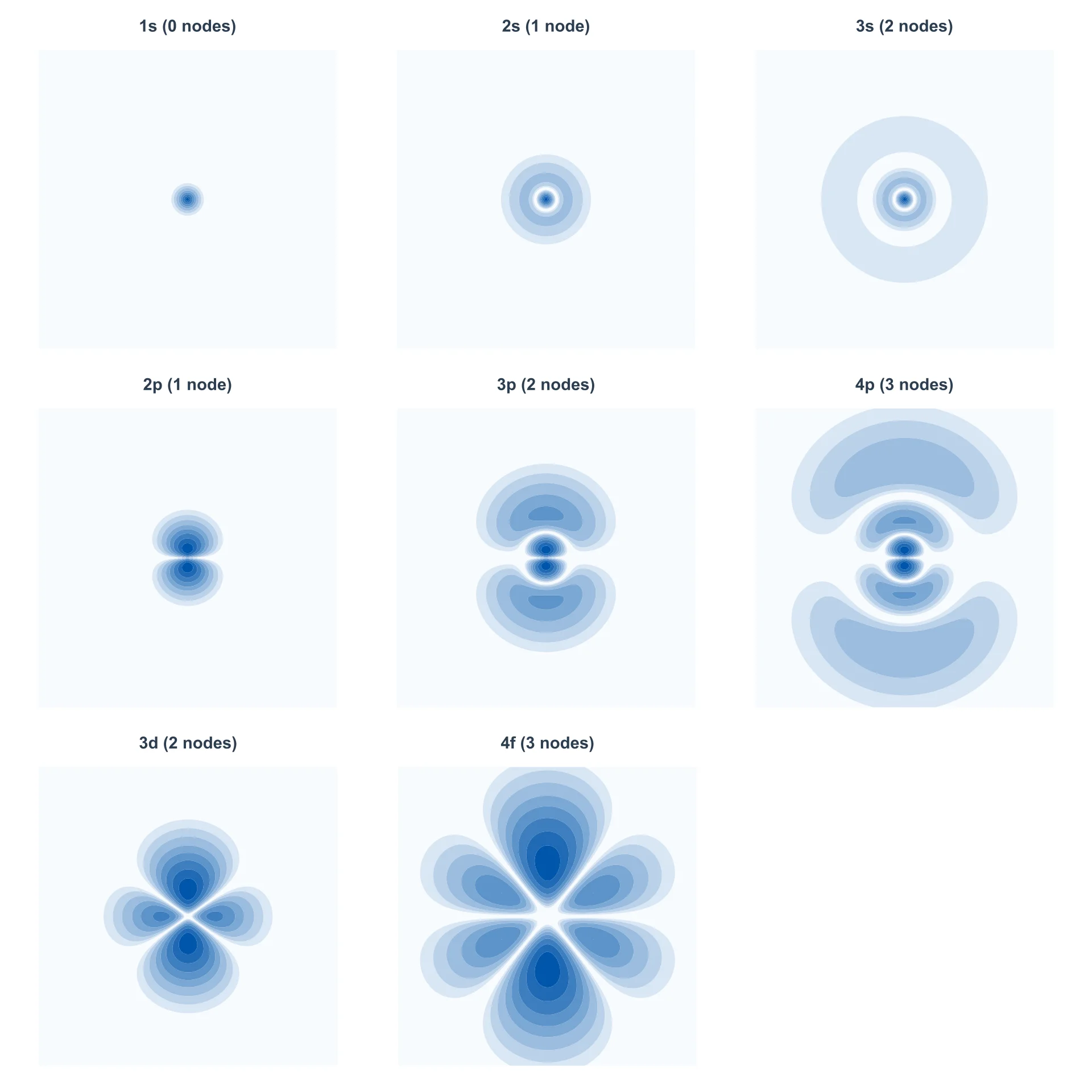
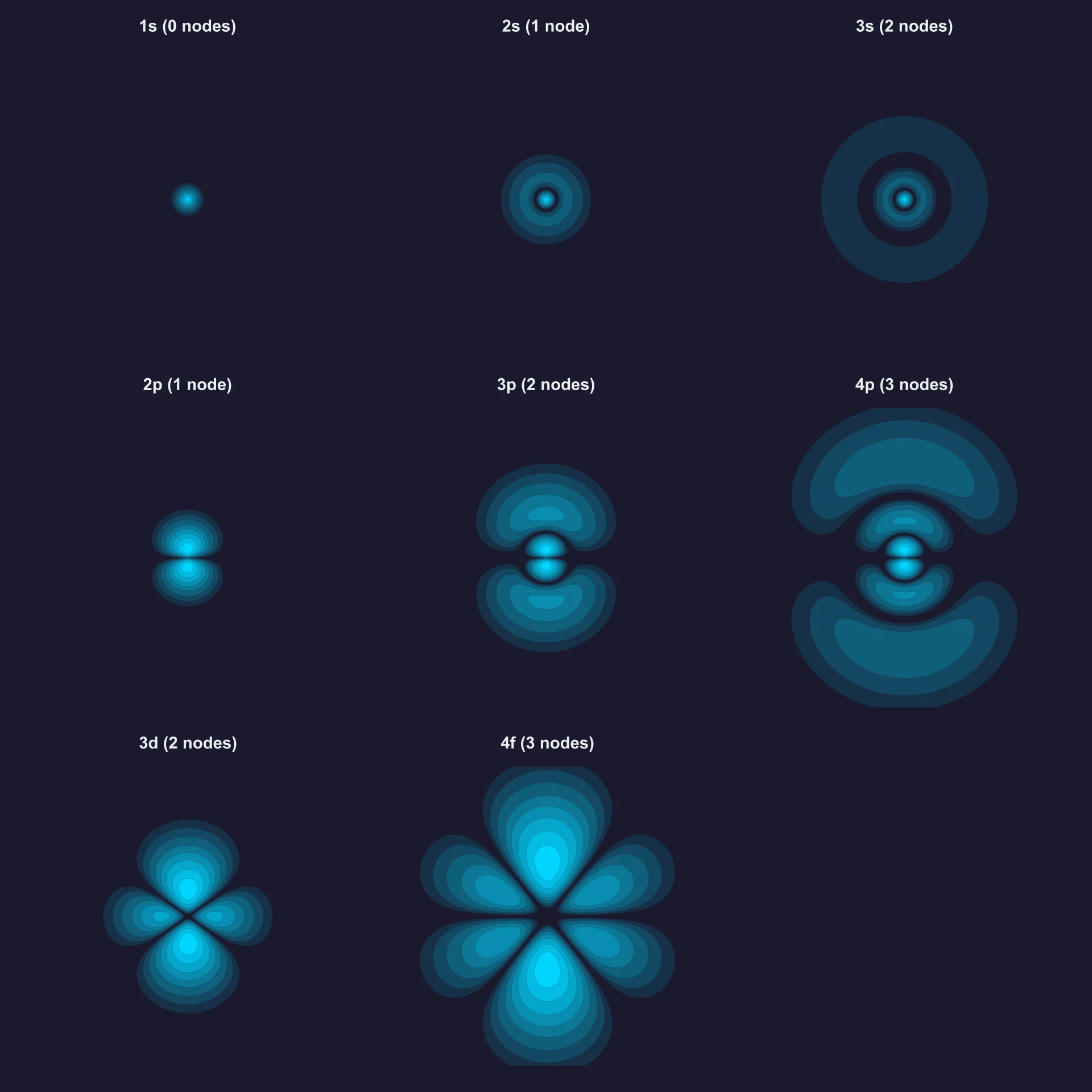
The cross-sections below show electron density for orbitals from 1s through 4f. Colored regions indicate high probability density, while nodes appear as gaps where the background shows through—radial nodes as circular gaps (spherical shells of zero probability) and angular nodes as linear gaps through the nucleus. All plots within each row use the same spatial scale for direct comparison.

Cross-sections showing nodes in atomic orbitals from 1s through 4f — Cross-sections of |Ψ|² in the xz-plane showing nodes for various orbitals. **Row 1:** s orbitals showing radial nodes as circular gaps. **Row 2:** p_z orbitals with the angular nodal plane at z = 0. **Row 3:** 3d_z² (2 angular nodes) and 4f_z³ (3 angular nodes). Each row uses a consistent spatial scale. Click to open with zoom controls.

In the s orbitals (top row), all nodes are radial. The 1s has no nodes, 2s has one ring of zero probability, and 3s has two. In the p orbitals (middle row), each has one angular node (the xy-plane where z = 0), plus additional radial nodes as n increases. The 3d_z² orbital has two angular nodal cones, while the 4f_z³ has three angular nodal surfaces.

Node Counter

Use this interactive tool to calculate the number of nodes for any orbital. Adjust the quantum numbers and watch the node counts update instantly.

viewof n_node = Inputs.range([1, 7], {
  step: 1,
  value: 3,
  label: "Principal quantum number (n)"
})

viewof l_node = Inputs.range([0, Math.min(n_node - 1, 3)], {
  step: 1,
  value: 0,
  label: "Angular momentum quantum number (l)"
})

node_counter_viz = {
  const width = 600;
  const height = 450;

  // Calculate nodes
  const radialNodes = n_node - l_node - 1;
  const angularNodes = l_node;
  const totalNodes = n_node - 1;

  // Orbital type label
  const orbitalTypes = ["s", "p", "d", "f"];
  const orbitalLabel = n_node + orbitalTypes[l_node];

  // Create SVG
  const svg = d3.create("svg")
    .attr("viewBox", [0, 0, width, height])
    .attr("class", "node-counter-svg")
    .style("max-width", `${width}px`)
    .style("height", "auto")
    .style("display", "block")
    .style("margin", "0 auto");

  // Background
  svg.append("rect")
    .attr("width", width)
    .attr("height", height)
    .attr("class", "node-bg");

  // Title
  svg.append("text")
    .attr("x", width / 2)
    .attr("y", 35)
    .attr("text-anchor", "middle")
    .attr("class", "node-title")
    .text(`Nodes in the ${orbitalLabel} orbital`);

  // Results box
  const boxY = 60;
  const boxHeight = 110;

  svg.append("rect")
    .attr("x", 40)
    .attr("y", boxY)
    .attr("width", width - 80)
    .attr("height", boxHeight)
    .attr("rx", 10)
    .attr("class", "results-box");

  // Node count results
  const results = [
    { label: "Radial nodes", formula: `${n_node} − ${l_node} − 1`, value: radialNodes },
    { label: "Angular nodes", formula: `${l_node}`, value: angularNodes },
    { label: "Total nodes", formula: `${n_node} − 1`, value: totalNodes }
  ];

  const colWidth = (width - 80) / 3;

  results.forEach((r, i) => {
    const cx = 40 + colWidth * (i + 0.5);

    svg.append("text")
      .attr("x", cx)
      .attr("y", boxY + 28)
      .attr("text-anchor", "middle")
      .attr("class", "result-label")
      .text(r.label);

    svg.append("text")
      .attr("x", cx)
      .attr("y", boxY + 62)
      .attr("text-anchor", "middle")
      .attr("class", "result-value")
      .text(r.value);

    svg.append("text")
      .attr("x", cx)
      .attr("y", boxY + 90)
      .attr("text-anchor", "middle")
      .attr("class", "result-formula")
      .text(`= ${r.formula}`);
  });

  // Visual representation
  const vizY = 200;
  const vizCenterX = width / 2;
  const vizSpacing = 130;

  // Draw radial nodes as concentric circles
  svg.append("text")
    .attr("x", vizCenterX - vizSpacing)
    .attr("y", vizY)
    .attr("text-anchor", "middle")
    .attr("class", "viz-label")
    .text("Radial nodes");

  const maxRadius = 80;
  const vizOffsetY = 90;

  for (let i = 0; i < radialNodes; i++) {
    const r = maxRadius * (i + 1) / (radialNodes + 1);
    svg.append("circle")
      .attr("cx", vizCenterX - vizSpacing)
      .attr("cy", vizY + vizOffsetY)
      .attr("r", r)
      .attr("class", "radial-node-circle");
  }

  // Nucleus dot
  svg.append("circle")
    .attr("cx", vizCenterX - vizSpacing)
    .attr("cy", vizY + vizOffsetY)
    .attr("r", 5)
    .attr("class", "nucleus-dot");

  // Outer boundary
  svg.append("circle")
    .attr("cx", vizCenterX - vizSpacing)
    .attr("cy", vizY + vizOffsetY)
    .attr("r", maxRadius)
    .attr("class", "boundary-circle");

  // Draw angular nodes as planes through nucleus
  svg.append("text")
    .attr("x", vizCenterX + vizSpacing)
    .attr("y", vizY)
    .attr("text-anchor", "middle")
    .attr("class", "viz-label")
    .text("Angular nodes");

  // Draw orbital shape outline
  svg.append("circle")
    .attr("cx", vizCenterX + vizSpacing)
    .attr("cy", vizY + vizOffsetY)
    .attr("r", maxRadius)
    .attr("class", "boundary-circle");

  // Angular node lines (planes viewed edge-on)
  if (angularNodes >= 1) {
    // First nodal plane (horizontal)
    svg.append("line")
      .attr("x1", vizCenterX + vizSpacing - maxRadius)
      .attr("x2", vizCenterX + vizSpacing + maxRadius)
      .attr("y1", vizY + vizOffsetY)
      .attr("y2", vizY + vizOffsetY)
      .attr("class", "angular-node-line");
  }
  if (angularNodes >= 2) {
    // Second nodal plane (vertical)
    svg.append("line")
      .attr("x1", vizCenterX + vizSpacing)
      .attr("x2", vizCenterX + vizSpacing)
      .attr("y1", vizY + vizOffsetY - maxRadius)
      .attr("y2", vizY + vizOffsetY + maxRadius)
      .attr("class", "angular-node-line");
  }
  if (angularNodes >= 3) {
    // Third nodal plane (diagonal)
    const offset = maxRadius * 0.707;
    svg.append("line")
      .attr("x1", vizCenterX + vizSpacing - offset)
      .attr("x2", vizCenterX + vizSpacing + offset)
      .attr("y1", vizY + vizOffsetY + offset)
      .attr("y2", vizY + vizOffsetY - offset)
      .attr("class", "angular-node-line");
  }

  // Nucleus dot for angular
  svg.append("circle")
    .attr("cx", vizCenterX + vizSpacing)
    .attr("cy", vizY + vizOffsetY)
    .attr("r", 5)
    .attr("class", "nucleus-dot");

  // Formulas at bottom
  svg.append("text")
    .attr("x", width / 2)
    .attr("y", height - 20)
    .attr("text-anchor", "middle")
    .attr("class", "formula-text")
    .html(`Radial = <tspan font-style="italic">n</tspan> − <tspan font-style="italic">l</tspan> − 1    •    Angular = <tspan font-style="italic">l</tspan>    •    Total = <tspan font-style="italic">n</tspan> − 1`);

  return svg.node();
}

node_counter_styles = html`
<style>
  /* Light mode */
  .node-counter-svg .node-bg {
    fill: #fafafa;
  }
  .node-counter-svg .node-title {
    fill: #1a1a1a;
    font-size: 18px;
    font-weight: bold;
  }
  .node-counter-svg .results-box {
    fill: #f0f4f8;
    stroke: #d0d7de;
    stroke-width: 1;
  }
  .node-counter-svg .result-label {
    fill: #666;
    font-size: 12px;
  }
  .node-counter-svg .result-value {
    fill: #2a30ec;
    font-size: 28px;
    font-weight: bold;
  }
  .node-counter-svg .result-formula {
    fill: #888;
    font-size: 11px;
    font-style: italic;
  }
  .node-counter-svg .viz-label {
    fill: #333;
    font-size: 12px;
    font-weight: 600;
  }
  .node-counter-svg .radial-node-circle {
    fill: none;
    stroke: #e74c3c;
    stroke-width: 2;
    stroke-dasharray: 4, 2;
  }
  .node-counter-svg .angular-node-line {
    stroke: #9b59b6;
    stroke-width: 2;
    stroke-dasharray: 4, 2;
  }
  .node-counter-svg .boundary-circle {
    fill: none;
    stroke: #ccc;
    stroke-width: 1;
  }
  .node-counter-svg .nucleus-dot {
    fill: #e74c3c;
  }
  .node-counter-svg .formula-text {
    fill: #666;
    font-size: 12px;
    font-style: italic;
  }

  /* Dark mode */
  body.quarto-dark .node-counter-svg .node-bg,
  .quarto-dark .node-counter-svg .node-bg,
  [data-bs-theme="dark"] .node-counter-svg .node-bg {
    fill: #0b0c14;
  }
  body.quarto-dark .node-counter-svg .node-title,
  .quarto-dark .node-counter-svg .node-title,
  [data-bs-theme="dark"] .node-counter-svg .node-title {
    fill: #e8ecf8;
  }
  body.quarto-dark .node-counter-svg .results-box,
  .quarto-dark .node-counter-svg .results-box,
  [data-bs-theme="dark"] .node-counter-svg .results-box {
    fill: #1a1d2e;
    stroke: #4a5072;
  }
  body.quarto-dark .node-counter-svg .result-label,
  .quarto-dark .node-counter-svg .result-label,
  [data-bs-theme="dark"] .node-counter-svg .result-label {
    fill: #a8afc7;
  }
  body.quarto-dark .node-counter-svg .result-value,
  .quarto-dark .node-counter-svg .result-value,
  [data-bs-theme="dark"] .node-counter-svg .result-value {
    fill: #00d9ff;
    filter: drop-shadow(0 0 4px rgba(0, 217, 255, 0.4));
  }
  body.quarto-dark .node-counter-svg .result-formula,
  .quarto-dark .node-counter-svg .result-formula,
  [data-bs-theme="dark"] .node-counter-svg .result-formula {
    fill: #6b7394;
  }
  body.quarto-dark .node-counter-svg .viz-label,
  .quarto-dark .node-counter-svg .viz-label,
  [data-bs-theme="dark"] .node-counter-svg .viz-label {
    fill: #e8ecf8;
  }
  body.quarto-dark .node-counter-svg .radial-node-circle,
  .quarto-dark .node-counter-svg .radial-node-circle,
  [data-bs-theme="dark"] .node-counter-svg .radial-node-circle {
    stroke: #ff6b6b;
    filter: drop-shadow(0 0 3px rgba(255, 107, 107, 0.4));
  }
  body.quarto-dark .node-counter-svg .angular-node-line,
  .quarto-dark .node-counter-svg .angular-node-line,
  [data-bs-theme="dark"] .node-counter-svg .angular-node-line {
    stroke: #c084fc;
    filter: drop-shadow(0 0 3px rgba(192, 132, 252, 0.4));
  }
  body.quarto-dark .node-counter-svg .boundary-circle,
  .quarto-dark .node-counter-svg .boundary-circle,
  [data-bs-theme="dark"] .node-counter-svg .boundary-circle {
    stroke: #4a5072;
  }
  body.quarto-dark .node-counter-svg .nucleus-dot,
  .quarto-dark .node-counter-svg .nucleus-dot,
  [data-bs-theme="dark"] .node-counter-svg .nucleus-dot {
    fill: #ff6b6b;
    filter: drop-shadow(0 0 4px rgba(255, 107, 107, 0.5));
  }
  body.quarto-dark .node-counter-svg .formula-text,
  .quarto-dark .node-counter-svg .formula-text,
  [data-bs-theme="dark"] .node-counter-svg .formula-text {
    fill: #6b7394;
  }
</style>
`

Orbital Shapes: A Summary

Combining the radial and angular parts gives the full three-dimensional orbital shape:

For interactive 3D visualizations of these orbital shapes, see the Atomic Orbitals Quick Reference.

Summary

Orbital Shapes

Each orbital type has a characteristic shape:

s orbitals: spherical
p orbitals: dumbbell (two lobes)
d orbitals: four lobes (cloverleaf) or donut + dumbbell (d_z²)
f orbitals: complex multi-lobed (six or eight lobes)

Orbital Size

Orbital size increases with principal quantum number n. A 3s orbital is much larger than a 1s orbital; a 3p is larger than a 2p. Higher n means higher energy and greater average distance from the nucleus.

Radial Probability Plots

The radial probability distribution shows where electrons are most likely to be found at various distances from the nucleus:

Peak position (most probable distance) increases with n
s orbitals have electron density at the nucleus; p, d, f do not

Nodes

Nodes are regions of zero probability:

Total nodes = n − 1
Radial nodes (spherical shells) = n − l − 1
Angular nodes (planes/cones) = l

Boundary Surfaces

The familiar orbital shapes in textbooks are boundary surfaces enclosing ~90 % of electron probability. Real orbitals are diffuse clouds with no sharp edges.

Interactive Orbital Visualization Tools

The orbital visualizations on this page are static representations. For interactive 3D exploration, several excellent free tools are available:

Orbital Viewer by David Manthey: A downloadable program for Windows that generates high-quality 3D orbital images with adjustable parameters.
ChemTube3D by the University of Liverpool: Browser-based 3D visualizations of atomic and molecular orbitals that you can rotate and explore.
Falstad Hydrogen Atom Applet by Paul Falstad: An interactive simulation showing probability distributions for hydrogen orbitals with adjustable quantum numbers.

These tools let you rotate orbitals, slice through probability distributions, and explore how quantum numbers affect orbital shapes in ways that static images cannot convey.

What’s Next

You now know what orbitals look like: their shapes, sizes, nodes, and probability distributions. The next question is: in what order do electrons fill these orbitals?

The answer determines an element’s chemistry. The Electron Configurations page covers the filling rules (Aufbau principle, Hund’s rule, Pauli exclusion) and explains why certain atoms like chromium and copper deviate from simple predictions. Understanding electron configurations is the key to understanding the periodic table itself.