Isotopes: Same Element, Different Mass

The identity of an element is determined by one thing and one thing only: the number of protons in its nucleus. This number, called the atomic number (Z), is the atom’s fundamental identifier. Every atom with 6 protons is a carbon atom; every atom with 92 protons is a uranium atom.

While the number of protons for any given element is fixed, the number of neutrons in the nucleus can vary. Atoms of the same element that have the same number of protons but different numbers of neutrons are called isotopes.

The Language of Isotopes: A/Z Notation

To describe a specific isotope unambiguously, chemists use a standard notation that provides all the necessary information about its subatomic composition. \[ {^A_Z}\mathrm{X} \] This notation is broken down as follows:

X is the symbol for the chemical element.
Z is the atomic number (the number of protons), written as a subscript to the left.
A is the mass number (the total number of protons + neutrons), written as a superscript to the left.

The number of neutrons can be easily calculated from this notation: #n = A − Z.

A Note on Notation

Sometimes you will see the subscript Z omitted (e.g., ¹⁴C). This is because the element symbol X already uniquely determines the atomic number. If the symbol is C, the atomic number must be 6. However, the full \({^A_Z}\mathrm{X}\) notation is the most complete and formal way to represent an isotope.

Concept Check 1:

What single characteristic determines an element’s identity?
How do isotopes of the same element differ from each other?
Write the notation for carbon-14, including its atomic number and mass number.

Solution

Number of protons
Different numbers of neutrons
¹⁴₆C

Properties and Abundance of Isotopes

Because isotopes have different numbers of neutrons, they have different mass numbers and therefore different masses. However, because they have the same number of protons and electrons, isotopes of an element have nearly identical chemical properties. They participate in chemical reactions in very similar ways.

The relative amount of each isotope found in a natural sample is known as its natural abundance. For example, protium (¹H) accounts for over 99.98% of all hydrogen atoms on Earth, while deuterium (²H) makes up most of the remainder. Tritium (³H) is so rare that its abundance is measured not as a percentage, but in trace amounts.

While most elements exist as a mixture of stable isotopes, 21 elements are monoisotopic, meaning they exist naturally as only a single isotope. IUPAC provides an authoritative list of these elements.

Quick Reference

See the table of Isotopic Masses and Natural Abundances for a list of common naturally occurring isotopes.

Example: The Isotopes of Carbon

Nearly all carbon on Earth is a mixture of two stable isotopes, with a third, radioactive isotope present in trace amounts. All three are carbon atoms because they each have 6 protons.

Carbon-12: This is the most common isotope (98.9% abundance). It has 6 protons and 6 neutrons.
- Mass Number (A) = 6p + 6n = 12
- Notation: \(^{12}_{\phantom{1}6}\mathrm{C}\)
Carbon-13: This stable isotope (1.1% abundance) has 6 protons and 7 neutrons.
- Mass Number (A) = 6p + 7n = 13
- Notation: \(^{13}_{\phantom{1}6}\mathrm{C}\)
Carbon-14: This is a rare, radioactive isotope (trace amounts) used in carbon dating. It has 6 protons and 8 neutrons.
- Mass Number (A) = 6p + 8n = 14
- Notation: \(^{14}_{\phantom{1}6}\mathrm{C}\)

The existence of these isotopes is why the atomic mass listed on the periodic table for carbon (12.01) is not a whole number. It is a weighted average of the masses of its naturally occurring isotopes, taking into account their different natural abundances.

Atomic Weight: A Technical Guide

In chemistry, we frequently use the value for an element’s “atomic mass” from the periodic table. While we often use this number in calculations as if it were a simple mass, it represents the culmination of a series of precise definitions and careful measurements. The distinction between relative isotopic mass, relative atomic mass (atomic weight), and the official standard atomic weight matters for understanding where that number comes from and what it actually represents.

The following sections cover the formal IUPAC definitions for these terms, the role of natural isotopic variation, and the relationship between the unitless values on the periodic table and the mass of an atom.

The Foundation: Relative Isotopic Mass

The starting point for all atomic mass measurements is the unified atomic mass unit (u), also known as the Dalton (Da). It is defined as exactly one-twelfth the mass of a single, unbound carbon-12 atom in its nuclear and electronic ground state.

\[1 \text{ u} = \frac{1}{12}~m_{\mathrm{a}}({}^{12}\text{C})\]

Here, m_a(¹²C) is the absolute mass of a carbon-12 atom. This specific quantity of mass is a fundamental physical constant known as the atomic mass constant (m_u). Therefore, the value of the atomic mass constant is

\[m_{\mathrm{u}} = 1 \text{ u} \approx 1.660~539~068~92(52) \times 10^{-27} \text{ kg}\]

From this standard, we can define the relative isotopic mass, A_r(ⁱE), for any isotope ^AE (where A is the mass number of element E). It is the ratio of the absolute mass of that isotope, m_a(^AE), to the atomic mass constant, m_u.

\[A_{\mathrm{r}}({}^A\mathrm{E}) = \frac{m_{\mathrm{a}}({}^A\mathrm{E})}{m_{\mathrm{u}}}\]

Because this is a ratio of two masses, the relative isotopic mass is a dimensionless quantity (it is unitless). For example, the relative isotopic mass of ³⁵Cl is 34.9688527, not 34.9688527 u.

The Weighted Average: Atomic Weight (Relative Atomic Mass)

Most elements in nature are not monoisotopic; they exist as a mixture of two or more stable isotopes. The atomic weight (or relative atomic mass) of an element E in a specific material P, denoted A_r(E)_P, is the weighted average of the relative isotopic masses of all the isotopes of that element in that specific sample. This quantity is what is most commonly meant by atomic weight.

The calculation, as defined by IUPAC, is:

\[A_{\mathrm{r}}(\mathrm{E})_{\text{P}} = \sum \left[ x({}^A\mathrm{E})_{\text{P}} ~ A_{\mathrm{r}}({}^A\mathrm{E}) \right]\]

In this equation:

The summation (Σ) is over all isotopes of element E.
x(^AE)_P is the amount fraction (also called isotopic abundance or mole fraction) of isotope ^AE in the specific material P.
A_r(^AE) is the relative isotopic mass of that isotope.

Like relative isotopic mass, the atomic weight A_r(E) is a dimensionless quantity.

The Challenge: Natural Isotopic Variation

The amount fractions, x(^AE), are not universal constants. As explained by the IUPAC Commission on Isotopic Abundances and Atomic Weights (CIAAW), the isotopic composition of an element can vary depending on its source due to mass-dependent fractionation in physical, chemical, and biological processes.

For example:

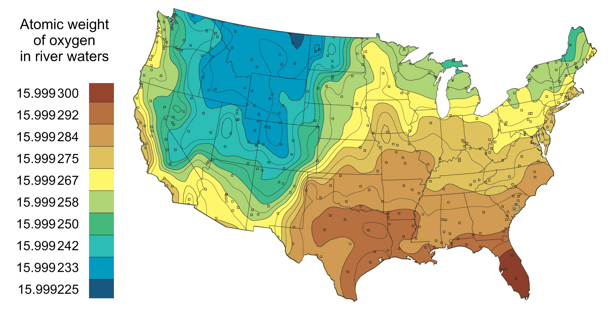
Oxygen in seawater has a slightly different ratio of ¹⁸O to ¹⁶O than oxygen in fresh polar water. This is because the lighter H₂¹⁶O evaporates more readily than the heavier H₂¹⁸O.
Carbon in the carbonate skeletons of marine organisms is isotopically different from the carbon in atmospheric CO₂.
Boron from marine carbonates has a different isotopic composition than boron from igneous rocks.

Because the atomic weight of an element depends on the isotopic abundances, and those abundances vary in nature, the atomic weight of boron from a rock in California might be slightly different from the atomic weight of boron from a mineral in Turkey.

Atomic Weight Variation for Oxygen

The atomic weight of elements such as oxygen can vary by region or specific material. Below is an image that shows the variation of atomic weight for oxygen across the continental US.

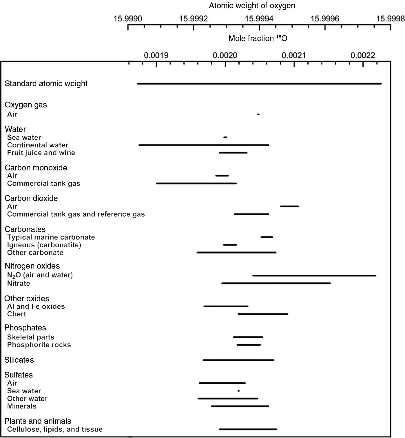
Variation in atomic weight of oxygen in river waters across the continental United States. Blue color indicates waters most depleted in <sup>18</sup>O (resulting in lower atomic weight of oxygen) and brown color indicates those most enriched in <sup>18</sup>O (resulting in higher atomic weight of oxygen). — Figure 1: Variation in atomic weight of oxygen in river waters across the continental United States. Blue color indicates waters most depleted in ¹⁸O (resulting in lower atomic weight of oxygen) and brown color indicates those most enriched in ¹⁸O (resulting in higher atomic weight of oxygen). Source: CIAAW

The figure below shows how the atomic weight of oxygen varies in different materials. This is due to varying compositions of oxygen isotopes in these materials.

Figure 2: Variation in atomic weight with isotopic composition of selected oxygen-bearing materials. Source: CIAAW

The Official Value: Standard Atomic Weight

To address this natural variation, IUPAC provides a single representative value for use in science, trade, and commerce: the standard atomic weight, A_r°(E).

The standard atomic weight is not a fundamental constant but a carefully evaluated expert opinion. The CIAAW determines this value by assessing all available measurements of isotopic abundances from normal terrestrial materials. This is the mass reported on a periodic table.

For many elements, the natural variation is significant enough that IUPAC expresses the standard atomic weight as an interval. For example, the standard atomic weight of boron is given as [10.806, 10.821]. For elements where the variation is smaller, IUPAC provides a single conventional atomic weight for practical use. For oxygen, this value is 15.999, with an uncertainty noted.

Applications of Isotopes

Isotopes have practical applications across medicine, environmental science, archaeology, and industry:

Medical Applications

Medical Imaging: Radioactive isotopes like technetium-99m are used in diagnostic scans to detect tumors and organ function
Cancer Treatment: Radioactive isotopes such as cobalt-60 and iodine-131 target and destroy cancer cells
Tracer Studies: Stable isotopes help track metabolic processes and drug distribution in the body

Environmental Applications

Climate Research: Oxygen isotope ratios in ice cores reveal past temperature changes
Water Tracing: Deuterium and oxygen-18 help track water movement through ecosystems
Pollution Sources: Carbon, nitrogen, and sulfur isotopes identify pollution origins

Archaeological and Geological Dating

Radiocarbon Dating: Carbon-14 dating determines ages of organic materials up to ~50,000 years
Geological Dating: Uranium-lead, potassium-argon, and other methods date rocks and minerals
Forensic Science: Isotope analysis helps determine geographic origins of materials

Industrial Applications

Food Preservation: Irradiation with cobalt-60 extends shelf life and kills pathogens
Quality Control: Isotope dilution mass spectrometry ensures accurate analytical measurements
Semiconductor Manufacturing: Isotopically pure silicon improves thermal conductivity in electronics

From Unitless Ratio to Physical Mass

How do we connect the dimensionless standard atomic weight on the periodic table to the actual mass of an atom? This is where the atomic mass constant, m_u, becomes essential.

The average mass of an atom, m_a°(E), of element E from terrestrial sources is the product of its standard atomic weight and the atomic mass constant, m_u:

\[\bar{m}_{\mathrm{a}}{^{\circ}}(\mathrm{E}) = A_{\mathrm{r}}{^{\circ}}(\mathrm{E}) \times m_{\mathrm{u}}\]

Since m_u = 1.660539… × 10⁻²⁷ kg, this calculation gives a result in kilograms.

However, for convenience, we almost always express atomic-scale masses in unified atomic mass units (u) or, equivalently, Daltons (Da). By definition, m_u = 1 u. Therefore, the average atomic mass of an element, expressed in units of u or Da, is numerically equal to its standard atomic weight.

The standard atomic weight of carbon, A_r°(C), is 12.011. It is a unitless ratio.
The average mass of a carbon atom in daltons is simply 12.011 u (or 12.011 Da).

This final step is an important convention that students sometimes miss. The number on the periodic table is a ratio, and it only becomes a mass with units when we explicitly multiply it by the atomic mass constant or, by convention, attach the units of u or Da.

Summary of Notation

Here is a table summarizing the notation introduced above that will be useful for the rest of this section.

Table 1: Symbols Used in Isotope Calculations

Concept Check 2:

Why is the atomic weight of carbon (12.01) not a whole number?
What is the difference between relative isotopic mass and relative atomic mass?
Why do some elements have atomic weights expressed as intervals?

Solution

It’s a weighted average of ¹²C and ¹³C masses
Relative isotopic mass is for a specific isotope, while relative atomic mass is the weighted average for an element
Natural isotopic variation exceeds measurement uncertainty

How to Calculate Atomic Weight

To calculate a weighted average for an element from a sample of isotopes, you need two pieces of information for each isotope:

The relative isotopic mass (A_r(^AE)) where superscript A is the mass number.
The natural abundance. This is the relative amount of that isotope found in a natural sample, typically expressed as a percent abundance (x(^AE) %) (e.g., 83.2 %).

The calculation itself is a sum of the contributions from each isotope. The result is the atomic weight of the element (A_r(E)). To perform the calculation, we must use the amount fraction (x(^AE)) of each isotope. The amount fraction (also called isotopic abundance or mole fraction) is simply the percent abundance divided by 100. For example, if an isotope’s percent abundance is 83.2 %, its amount fraction is 0.832.

Using formal notation, the calculation for an element (E) with n isotopes is

\[A_{\mathrm{r}} ( \mathrm{E} ) = \sum_{i=1}^n ~\biggl[ x (^A\mathrm{E} ) ~ A_{\mathrm{r}} ( ^A\mathrm{E} ) \biggr]_i\]

where i indexes the isotopes, each with mass number A_i.

It is important to remember that the percent abundances of all naturally occurring isotopes for an element must add up to 100%, and their amount fractions must sum to 1.

Note that these calculations in general chemistry generally have you assume that the atomic weight is approximately equal to the standard atomic weight for an element. Therefore, you may generally treat these values to be the same.

\[A_{\mathrm{r}}(\mathrm{E}) \approx A_{\mathrm{r}}{^{\circ}}(\mathrm{E})\]

This allows you to use the standard atomic weight of an element reported on the periodic table as the atomic weight for the element you are using in these calculations.

Example: Atomic Weight of Boron

Boron has a reported standard atomic weight (A_r°(B)) of 10.81. However, boron naturally exists as two isotopes. Boron-11 is the most abundant isotope of boron with a percent abundance of 80.1 %.

Solution

First, recognize that the table above provides the atomic mass (m_a(^AB)) (in u) of each specific isotope. These quantities are numerically equivalent to the relative isotopic mass A_r(^AE) (dimensionless).

Calculate the atomic weight of boron (A_r(B)). Since there are two naturally occurring isotopes for boron, we must sum two terms together in our calculation (n = 2).

\[ \begin{align*} A_{\mathrm{r}} (\mathrm{E}) &= \sum_{i=1}^n ~\biggl[ x (^A\mathrm{E}) ~ A_{\mathrm{r}} (^A\mathrm{E}) \biggr]_i \\[1.5ex] A_{\mathrm{r}}(\mathrm{B}) &= \Bigl [ x \! \left ( \mathrm{^{10}B} \right ) ~ A_{\mathrm{r}} \! \left (\mathrm{^{10}B} \right ) \Bigr ] + \Bigl [ x \! \left (\mathrm{^{11}B} \right ) ~ A_{\mathrm{r}} \! \left (\mathrm{^{11}B}\right ) \Bigr ] \\[1.5ex] &= \left ( 0.19\bar{9}\right ) \left ( 10.012936\bar{9} \right ) + \left ( 0.80\bar{1} \right ) \left ( 11.009305\bar{4} \right ) \\[1.5ex] &= 1.9\bar{9}25 + 8.8\bar{1}84\\[1.5ex] &= 10.8\bar{1}09 \\[1.5ex] &= 10.81 \end{align*} \]

Common Pitfalls in Isotope Calculations

Algebraic Mistakes

Distribution Errors: Remember to distribute negative signs: −(a+b) = −a−b, not −(a+b) = −a+b
Order of Operations: Calculate weighted averages before final rounding
Variable Isolation: When solving for unknown abundances, ensure all terms are properly isolated

Precision and Rounding Mistakes

Premature Rounding: Keep guard digits in intermediate calculations, round only at the end
Significant Figure Mismatch: Final answers should match the precision of your least precise input
Unit Confusion: Remember that atomic weights are dimensionless, but atomic masses have units (u)

Conceptual Mistakes

Mixing A_r and A_r°: Use standard atomic weights (periodic table values) as approximations for specific sample atomic weights
Amount vs. Percentage: Remember to convert between amount fractions (decimal) and percent abundances (%)
Forgetting the Sum Check: Always verify that percent abundances sum to 100 %

Calculation Strategy

Method 1 vs. Method 2: When possible, use the “sum to 100 %” method for finding missing abundances rather than working backward from atomic weight
Choose Your Unknown: When solving for multiple unknowns, pick the easier one to isolate first

Practice: Atomic Weight of Lithium

Determine the relative atomic weight of lithium using the isotopic data for lithium found on the Isotopic Masses and Natural Abundances quick reference page.

Solution

Isotope Data for Li

Calculate the atomic weight for Li

There are two naturally occurring isotopes for Lithium (n = 2). Therefore, we will need to sum together two terms in our calculation.

\[ \begin{align*} A_{\mathrm{r}} ( \mathrm{E} ) &= \sum_{i=1}^n ~\biggl[ x(^A\mathrm{E} ) ~ A_{\mathrm{r}} (^A\mathrm{E} ) \biggr]_i \\[1.5ex] A_{\mathrm{r}}(\mathrm{Li}) &= \Bigl [ x( \mathrm{^{6}Li}) ~ A_{\mathrm{r}} (\mathrm{^{6}Li} ) \Bigr ] + \Bigl [ x (\mathrm{^{7}Li} ) ~ A_{\mathrm{r}} ( \mathrm{^{7}Li} ) \Bigr ] \\[1.5ex] &= ( 0.075\bar{9} ) ( 6.015122887\bar{4} ) + ( 0.924\bar{1} ) ( 7.01600343\bar{7} ) \\[1.5ex] &= 0.45\bar{6}55 + 6.48\bar{3}49\\[1.5ex] &= 6.94\bar{0}04 \\[1.5ex] &= 6.940 \end{align*} \]

Calculating Percent Abundance

We can find the percent abundance for an isotope algebraically given a different set of starting information. There are two different methods you can use for this, one being more precise than the other.

Example: Calculating One Percent Abundance for Oxygen

Sometimes you will be tasked with finding the percent abundance of a particular isotope. Consider the isotope data for oxygen.

Find the percent abundance of oxygen-18. There are two methods for doing this.

Method 1: Sum to 100 % (most precise)

The simplest and most direct method relies on a fundamental rule: the percent abundances of all naturally occurring isotopes for an element must sum to 100%. Since we know the abundances for oxygen-16 and oxygen-17, we can find the abundance of oxygen-18 by simple subtraction.

\[ \begin{align*} 100~\% &= x(^{16}\mathrm{O})~\% + x(^{17}\mathrm{O})~\% + x(^{18}\mathrm{O})~\% \longrightarrow \\[1.5ex] x(^{18}\mathrm{O})~\% &= 100~\% - \Bigl [ x(^{16}\mathrm{O})~\% + x(^{17}\mathrm{O})~\% \Bigr ] \\[1.5ex] &= 100~\% - (99.75\bar{7} + 0.03\bar{8})~\% \\[1.5ex] &= 0.205~\% \end{align*} \]

Method 2: Working Backward from Atomic Weight (less precise)

First, we can refer to the periodic table to find the standard atomic weight of oxygen (A_r^°(O) = 16.00) to use as our atomic weight for oxygen (A_r(O)) for this calculation. This value is imprecise as it is rounded to two decimal places; therefore, our final answer will have rounding error in it and will not exactly be 0.205 %.

Next, we write out our equation and expand. Since we have three isotopes for oxygen, n = 3, meaning we sum together three terms. Next, we rearrange for the amount fraction of oxygen-18 term (x(¹⁸O)) and then solve for the amount fraction of oxygen-18.

Finally we convert amount fraction to percent abundance.

\[ \begin{align*} x (^{18}\mathrm{O} )~\% &= x (^{18}\mathrm{O} ) \times 100~\% \\[1.5ex] &= 0.00\bar{2}08 \times 100~\% \\[1.5ex] &= 0.\bar{2}08~\% \\[1.5ex] &= 0.2~\% \end{align*} \]

Which Method to Use?

Method 1 is more precise because it relies only on the given percent abundances, which must sum to exactly 100%. Method 2 introduces rounding error because the atomic weight from the periodic table (16.00 u) is itself rounded. In this case, Method 2 gives 0.2 %, while Method 1 gives the more accurate 0.205 %. The difference is small here, but for elements with greater natural isotopic variation or when using heavily rounded data, the error can be larger. If you have a choice, use Method 1 for the most accurate result.

Example: Two Percent Abundances for Oxygen

We can approximate two percent abundances for oxygen. For this exercise, we must use a very precise atomic weight for oxygen. Using the value given in the periodic table is too imprecise to use with the very precise isotope data below. For this example, use 15.99940911 for the atomic weight of oxygen.

Provided is the isotope data for oxygen. Notice how two percent abundance values are missing.

Caution: Challenging Problem Ahead

This type of problem is not for the faint of heart. It is meant to challenge your algebraic skills and some teachers may not even have you perform this type of calculation given the effort required to solve it. However, it is a great test of how well you know your algebra and will only strengthen your ability to solve future problems throughout the course!

I highly recommend working these things out on paper and to work very methodically through the math. This will ensure that you do not make mistakes.

Finally, this example problem uses very accurate scientific data which requires you to use numbers with great precision (many decimal places). This, and tracking significant figures, will also slow you down immensely.

However, obtaining the final result is very satisfying as you are calculating numbers with high precision! Do not let the complexity of this problem discourage you from putting your algebra and chemistry knowledge to the test!

If you are able to solve this type of problem, take a long break and treat yourself!

Solution

First, we recognize that the percent abundance for each isotope must sum to exactly 100 %.

\[ 100~\% = x(^{16}\mathrm{O})~\% + x(^{17}\mathrm{O})~\% + x(^{18}\mathrm{O})~\% \]

It will be convenient for us to represent this as amount fraction. Therefore, the amount fraction of each isotope must sum to exactly 1.

\[ 1 = x(^{16}\mathrm{O}) + x(^{17}\mathrm{O}) + x(^{18}\mathrm{O}) \]

We have the amount fraction for oxygen-16. This can be done in different ways. I will show one way below. We can determine the remaining two by solving for the amount fraction of one of the unknowns (say for oxygen-17) and then, with some substitution, determine the second unknown (oxygen-18).

Step 1: Find for the amount fraction of oxygen-17 in terms of oxygen-18

\[ \begin{align*} 1 &= x(^{16}\mathrm{O}) + x(^{17}\mathrm{O}) + x(^{18}\mathrm{O}) \longrightarrow \\[1.5ex] x(^{17}\mathrm{O}) &= 1 - x(^{16}\mathrm{O}) - x(^{18}\mathrm{O}) \\[1.5ex] &= 1 - 0.9975\bar{7} - x(^{18}\mathrm{O}) \\[1.5ex] &= 0.0024\bar{3} - x(^{18}\mathrm{O}) \end{align*} \]

Step 2: Substitute in the fraction amount for oxygen-17 and solve for oxygen-18

Now write out our equation in terms of amount fractions and relative isotopic masses and set it equal to the provided standard atomic weight of oxygen (A_r(O) = 15.99940911).

We will have to:

Substitute in the amount fraction expression for oxygen-17 (x(¹⁷O)) from Step 1; shown in red).
Distribute the atomic weight of oxygen-17 (A_r(¹⁷O)) into this expression (shown in green).
Solve for the amount fraction of oxygen-18 (x(¹⁸O)). You will have to factor out the amount fraction of oxygen-18 (shown in purple).

Given that there are three isotopes, we must sum together three terms (n = 3).

\[ \begin{align*} A_{\mathrm{r}} ( \mathrm{E} ) &= \sum_{i=1}^n ~\biggl[ x (^A\mathrm{E} ) ~ A_{\mathrm{r}} (^A\mathrm{E} ) \biggr]_i \\[1.5ex] A_{\mathrm{r}}(\mathrm{O}) &= \Bigl[ x (^{16}\mathrm{O}) ~ A_{\mathrm{r}} (^{16}\mathrm{O}) \Bigr] + \Bigl[ {\color{red}x (^{17}\mathrm{O} )} ~ A_{\mathrm{r}}(^{17}\mathrm{O}) \Bigr] + \Bigl[ x (^{18}\mathrm{O}) ~ A_{\mathrm{r}} (^{18}\mathrm{O}) \Bigr] \\[1.5ex] A_{\mathrm{r}}(\mathrm{O}) &= \Bigl[ x(^{16}\mathrm{O}) ~ A_{\mathrm{r}}(^{16}\mathrm{O}) \Bigr] + \biggl\{ \Bigl [ {\color{red}0.0024\bar{3} - x(^{18}\mathrm{O})} \Bigr ] ~ {\color{green}A_{\mathrm{r}}(^{17}\mathrm{O})} \biggr\} + \Bigl[ x(^{18}\mathrm{O}) ~ A_{\mathrm{r}}(^{18}\mathrm{O}) \Bigr] \\[1.5ex] A_{\mathrm{r}}(\mathrm{O}) &= \Bigl[ x(^{16}\mathrm{O}) ~ A_{\mathrm{r}}(^{16}\mathrm{O}) \Bigr] + \Bigl[ 0.0024\bar{3}~{\color{green}A_{\mathrm{r}}(^{17}\mathrm{O})}\Bigr ] - \Bigl[ x(^{18}\mathrm{O})~{\color{green}A_{\mathrm{r}}(^{17}\mathrm{O})} \Bigr] + \Bigl[ x(^{18}\mathrm{O}) ~ A_{\mathrm{r}}(^{18}\mathrm{O}) \Bigr] \\[1.5ex] A_{\mathrm{r}}(\mathrm{O}) + \Bigl [ {\color{purple} x(^{18}\mathrm{O})}~A_{\mathrm{r}}(^{17}\mathrm{O}) \Bigr] - \Bigl[ {\color{purple} x(^{18}\mathrm{O})} ~ A_{\mathrm{r}}(^{18}\mathrm{O}) \Bigr] &= \Bigl[ x(^{16}\mathrm{O}) ~ A_{\mathrm{r}}(^{16}\mathrm{O}) \Bigr] + \Bigl[ 0.0024\bar{3}~A_{\mathrm{r}}(^{17}\mathrm{O}) \Bigr ] \\[1.5ex] A_{\mathrm{r}}(\mathrm{O}) + {\color{purple} x(^{18}\mathrm{O})} \Bigl [ A_{\mathrm{r}}(^{17}\mathrm{O}) - A_{\mathrm{r}}(^{18}\mathrm{O}) \Bigr ] &= \Bigl[ x(^{16}\mathrm{O}) ~ A_{\mathrm{r}}(^{16}\mathrm{O}) \Bigr] + \Bigl[ 0.0024\bar{3}~A_{\mathrm{r}}(^{17}\mathrm{O}) \Bigr ] \\[1.5ex] x(^{18}\mathrm{O}) &= \biggl\{ \Bigl[ x(^{16}\mathrm{O}) ~ A_{\mathrm{r}}(^{16}\mathrm{O}) \Bigr] + \Bigl[ 0.0024\bar{3}~A_{\mathrm{r}}(^{17}\mathrm{O}) \Bigr ] - A_{\mathrm{r}}(\mathrm{O}) \biggr\} ~ \Bigl [ A_{\mathrm{r}}(^{17}\mathrm{O}) - A_{\mathrm{r}}(^{18}\mathrm{O}) \Bigr ]^{-1}\\[1.5ex] &= \biggl\{ \Bigl[ (0.9975\bar{7}) (15.9949146195\bar{7}) \Bigr] + \Bigl[ ( 0.0024\bar{3}) ( 16.999131756\bar{5}) \Bigr ] - 15.9994091\bar{1} \biggr\} ~ \Bigl( 16.999131756\bar{5} - 17.999159612\bar{9} \Bigr)^{-1}\\[1.5ex] &= (15.95\bar{6}05 + 0.041\bar{3}08 - 15.9994091\bar{1})~ ( -1.000027856\bar{4})^{-1} \\[1.5ex] &= ( -0.00\bar{2}05111 ) ( -1.000027856\bar{4} )^{-1} \\[1.5ex] &= 0.00\bar{2}05 \end{align*} \]

Why Such High Precision?

Notice in the numerator that we’re adding two contributions (15.95605 + 0.041308) and then subtracting a very similar number (15.99940911), resulting in the tiny value −0.00205111. This is an example of catastrophic cancellation. When you subtract nearly equal numbers, small rounding errors in the inputs become amplified in the result.

This happens here because oxygen is 99.757 % oxygen-16, so we’re solving for a tiny difference. This makes the calculation extremely sensitive to precision, which is why using the rounded periodic table value (16.00) would fail completely, as shown in the callout below.

Step 3: Convert the amount fraction of oxygen-18 into percent abundance

\[ \begin{align*} x (^{18}\mathrm{O} )\% &= x(^{18}\mathrm{O}) \times 100~\% \\[1.5ex] &= 0.00\bar{2}05 \times 100~\% \\[1.5ex] &= 0.\bar{2}05~\% \\[1.5ex] &= 0.2~\% \end{align*} \]

Step 4: Solve for the percent abundance of oxygen-17

Now that we know the percent abundance for oxygen-16 and oxygen-18, we can now solve for the percent abundance of oxygen-17. Note that you must use the unrounded number from Step 3 for this calculation (see rules for Multi-Step Calcuations in the Significant Figures section).

\[ \begin{align*} 100~\% &= x(^{16}\mathrm{O}) \% + x(^{17}\mathrm{O}) \% + x(^{18}\mathrm{O}) \% \longrightarrow \\[1.5ex] x(^{17}\mathrm{O})~\% &= 100~\% - x(^{16}\mathrm{O})~\% - x(^{18}\mathrm{O})~\% \\[1.5ex] &= 100~\% - 99.75\bar{7}~\% -0.\bar{2}05~\% \\[1.5ex] &=0.\bar{0}38 ~\% \end{align*} \]

Why Did We Use a Provided Atomic Weight?

In this problem, you were given a very precise standard atomic weight (15.99940911) instead of being asked to use the value from the periodic table (typically shown as 16.00 or 15.999). This precision was essential because of the catastrophic cancellation discussed above.

When solving for isotopic abundances algebraically, we’re calculating small differences between large, nearly-equal numbers. Any rounding error in the atomic weight gets amplified dramatically in the final answer. The provided value of 15.99940911 is the true weighted average calculated from the high-precision isotopic masses and accepted natural abundances, ensuring our algebra works backward correctly.

What happens if we use the periodic table value?

If we had used the rounded atomic weight of 16.00, the calculation would yield x(¹⁸O) = 0.264 %. Substituting this back to find x(¹⁷O) gives:

\[100~\% - 99.757~\% - 0.264~\% = -0.021~\%\]

A negative abundance is physically impossible. This nonsensical result occurs because the rounded value (16.00) has insufficient precision for this type of calculation. The rounding error is small in absolute terms (≈0.001 u), but when amplified by the subtraction of nearly-equal numbers, it completely destroys the calculation.

Periodic table values work well for most stoichiometric calculations where we work forward from atomic weights to molar masses. However, when working backward to solve for isotopic abundances or other fine details, you need data with precision that matches the scale of the quantity you’re solving for.

Note: Many instructors simplify these problems by providing less precise isotopic data (rounded to 2-3 decimal places), which allows you to use periodic table values and speeds up the algebra considerably. The trade-off is that your answers approximate the true natural abundances rather than matching them exactly.

Practice: Two Percent Abundances for Silicon

Determine the two unknown percent abundances for silicon. Refer to the periodic table for the standard atomic weight of silicon (A_r°(Si)), which you will use as the approximate atomic weight (A_r(Si)) in your calculation.

Note: This problem purposefully uses less precise data for compactness. This is a realistic treatment of this type of problem in a typical course.

Solution

Step 1: Find for the amount fraction of silicon-29 in terms of silicon-30

\[ \begin{align*} 1 &= x(^{28}\mathrm{Si}) + x(^{29}\mathrm{Si}) + x(^{30}\mathrm{Si}) \longrightarrow \\[1.5ex] x(^{29}\mathrm{Si}) &= 1 - x(^{28}\mathrm{Si}) - x(^{30}\mathrm{Si}) \\[1.5ex] &= 1 - 0.922\bar{2} - x(^{30}\mathrm{Si}) \\[1.5ex] &= 0.077\bar{8} - x(^{30}\mathrm{Si}) \end{align*} \]

Step 2: Substitute in the fraction amount for silicon-29 and solve for silicon-30

Now write out our equation in terms of amount fractions and relative isotopic masses and set it equal to the atomic weight of silicon (A_r(Si) = 28.09).

Key Points:

Substitute in the amount fraction expression for silicon-29 (x(²⁹Si)) from Step 1; shown in red).
Distribute the atomic weight of silicon-29 (A_r(²⁹Si)) into this expression (shown in green).
Solve for the amount fraction of silicon-30 (x(³⁰Si)). You will have to factor out the amount fraction of silicon-30 (shown in purple).

Given that there are three isotopes, we must sum together three terms (n = 3).

\[ \begin{align*} A_{\mathrm{r}}(\mathrm{E}) &= \sum_{i=1}^n ~\biggl[ x(^A\mathrm{E}) ~ A_{\mathrm{r}}(^A\mathrm{E}) \biggr]_i \\[1.5ex] A_{\mathrm{r}}(\mathrm{Si}) &= \Bigl[ x(^{28}\mathrm{Si}) ~ A_{\mathrm{r}}(^{28}\mathrm{Si}) \Bigr] + \Bigl[ {\color{red}x(^{29}\mathrm{Si})} ~ A_{\mathrm{r}}(^{29}\mathrm{Si}) \Bigr] + \Bigl[ x(^{30}\mathrm{Si}) ~ A_{\mathrm{r}}(^{30}\mathrm{Si}) \Bigr] \\[1.5ex] A_{\mathrm{r}}(\mathrm{Si}) &= \Bigl[ x(^{28}\mathrm{Si}) ~ A_{\mathrm{r}}\left (^{28}\mathrm{Si}\right ) \Bigr] + \biggl\{ \Bigl [ {\color{red}0.077\bar{8} - x(^{30}\mathrm{Si})} \Bigr ] ~ {\color{green}A_{\mathrm{r}}(^{29}\mathrm{Si})} \biggr\} + \Bigl[ x(^{30}\mathrm{Si}) ~ A_{\mathrm{r}}(^{30}\mathrm{Si}) \Bigr] \\[1.5ex] A_{\mathrm{r}}(\mathrm{Si}) &= \Bigl[ x(^{28}\mathrm{Si}) ~ A_{\mathrm{r}}(^{28}\mathrm{Si}) \Bigr] + \Bigl[ 0.077\bar{8}~{\color{green}A_{\mathrm{r}}(^{29}\mathrm{Si})}\Bigr ] - \Bigl[ x(^{30}\mathrm{Si})~{\color{green}A_{\mathrm{r}}(^{29}\mathrm{Si})} \Bigl] + \Bigl[ x(^{30}\mathrm{Si}) ~ A_{\mathrm{r}}(^{30}\mathrm{Si}) \Bigr] \\[1.5ex] A_{\mathrm{r}}(\mathrm{Si}) + \Bigl [ {\color{purple} x(^{30}\mathrm{Si})}~A_{\mathrm{r}}(^{29}\mathrm{Si}) \Bigr] - \Bigl[ {\color{purple} x(^{30}\mathrm{Si})} ~ A_{\mathrm{r}}(^{30}\mathrm{Si}) \Bigr] &= \Bigl[ x(^{28}\mathrm{Si}) ~ A_{\mathrm{r}}(^{28}\mathrm{Si}) \Bigr] + \Bigl[ 0.077\bar{8}~A_{\mathrm{r}}(^{29}\mathrm{Si}) \Bigr ] \\[1.5ex] A_{\mathrm{r}}(\mathrm{Si}) + {\color{purple} x(^{30}\mathrm{Si})} \Bigl [ A_{\mathrm{r}}(^{29}\mathrm{Si}) - A_{\mathrm{r}}(^{30}\mathrm{Si}) \Bigr ] &= \Bigl[ x(^{28}\mathrm{Si}) ~ A_{\mathrm{r}}(^{28}\mathrm{Si}) \Bigr] + \Bigl[ 0.077\bar{8}~A_{\mathrm{r}}(^{29}\mathrm{Si}) \Bigr ] \\[1.5ex] x(^{30}\mathrm{Si}) &= \biggl\{ \Bigl[ x(^{28}\mathrm{Si}) ~ A_{\mathrm{r}}(^{28}\mathrm{Si}) \Bigr] + \Bigl[ 0.077\bar{8}~A_{\mathrm{r}}(^{29}\mathrm{Si}) \Bigr ] - A_{\mathrm{r}}(\mathrm{Si}) \biggr\} ~ \Bigl [ A_{\mathrm{r}}(^{29}\mathrm{Si}) - A_{\mathrm{r}}(^{30}\mathrm{Si}) \Bigr ]^{-1}\\[1.5ex] &= \biggl\{ \Bigl[ (0.922\bar{2}) (27.9\bar{8}) \Bigr] + \Bigl[ (0.077\bar{8}) (28.9\bar{8}) \Bigr ] - 28.0\bar{9} \biggr\} ~ \Bigl( 28.9\bar{8} - 29.9\bar{7} \Bigr)^{-1}\\[1.5ex] &= ( 25.8\bar{0}32 + 2.2\bar{5}46 - 28.0\bar{9})~ ( -0.9\bar{9}00)^{-1} \\[1.5ex] &= ( -0.0\bar{3}22) ( -0.9\bar{9}00)^{-1} \\[1.5ex] &= 0.0\bar{3}25 \end{align*} \]

Step 3: Convert the amount fraction of silicon-30 into percent abundance

\[ \begin{align*} x \left (^{30}\mathrm{Si} \right )\% &= x(^{30}\mathrm{Si}) \times 100~\% \\[1.5ex] &= 0.0\bar{3}25 \times 100~\% \\[1.5ex] &= \bar{3}.25~\% \\[1.5ex] &= 3~\% \end{align*} \]

Step 4: Solve for the percent abundance of silicon-29

Now that we know the percent abundance for silicon-28 and silicon-30, we can now solve for the percent abundance of silicon-29. Note that you must use the unrounded number from Step 3 for this calculation (see rules for Multi-Step Calcuations in the Significant Figures section).

\[ \begin{align*} 100~\% &= x(^{28}\mathrm{Si})~\% + x(^{29}\mathrm{Si}) \% + x(^{30}\mathrm{Si}) \% \longrightarrow \\[1.5ex] x(^{29}\mathrm{Si}) \% &= 100~\% - x(^{28}\mathrm{Si})~\% - x(^{30}\mathrm{Si})~\% \\[1.5ex] &= 100~\% - 92.2\bar{2}~\% - \bar{3}.25~\% \\[1.5ex] &= \bar{4}.53~\% \\[1.5ex] &= 4~\% \end{align*} \]

We have done a good job approximating the two unknown percent abundances. Compare them to the actual percent abundances determined from more precise isotope data.

Other Types of Percent Abundance Problems

Given the algebraic nature of these problems, you may encounter similar exercises where you solve for some unknown atomic mass(es). For these, all the percent abundances are provided while a mass or two are not provided.

Extra Practice

These practice problems provide the answers but not the worked out solutions.

The reported isotopic data has been rounded sufficiently to allow you to use the standard atomic weight given on the periodic table (to two decimal places).
The reported answers are corrected for these imprecise data but will not match experimental data.

Practice: Two Percent Abundances for Argon

Determine the percent abundance (to one decimal place) for argon-38 and argon-40. Refer to the periodic table for the standard atomic weight of argon (A_r°(Ar)), which you will use as the approximate atomic weight (A_r(Ar)) in your calculation.

Solution

x(³⁸Ar) % = 1.8 %
x(⁴⁰Ar) % = 97.8 %